RNA_DGE_Comp_Species_Ensemble
2026-01-27
Last updated: 2026-02-20
Checks: 7 0
Knit directory: CrossSpecies_CM_Diff_RNA/
This reproducible R Markdown analysis was created with workflowr (version 1.7.2). The Checks tab describes the reproducibility checks that were applied when the results were created. The Past versions tab lists the development history.
Great! Since the R Markdown file has been committed to the Git repository, you know the exact version of the code that produced these results.
Great job! The global environment was empty. Objects defined in the global environment can affect the analysis in your R Markdown file in unknown ways. For reproduciblity it’s best to always run the code in an empty environment.
The command set.seed(20251129) was run prior to running
the code in the R Markdown file. Setting a seed ensures that any results
that rely on randomness, e.g. subsampling or permutations, are
reproducible.
Great job! Recording the operating system, R version, and package versions is critical for reproducibility.
Nice! There were no cached chunks for this analysis, so you can be confident that you successfully produced the results during this run.
Great job! Using relative paths to the files within your workflowr project makes it easier to run your code on other machines.
Great! You are using Git for version control. Tracking code development and connecting the code version to the results is critical for reproducibility.
The results in this page were generated with repository version 8bce9df. See the Past versions tab to see a history of the changes made to the R Markdown and HTML files.
Note that you need to be careful to ensure that all relevant files for
the analysis have been committed to Git prior to generating the results
(you can use wflow_publish or
wflow_git_commit). workflowr only checks the R Markdown
file, but you know if there are other scripts or data files that it
depends on. Below is the status of the Git repository when the results
were generated:
Ignored files:
    Ignored:    .Rhistory
    Ignored:    .Rproj.user/
    Ignored:    data/
Note that any generated files, e.g. HTML, png, CSS, etc., are not included in this status report because it is ok for generated content to have uncommitted changes.
These are the previous versions of the repository in which changes were
made to the R Markdown
(analysis/RNA_DGE_Comp_Species_Ensemble.Rmd) and HTML
(docs/RNA_DGE_Comp_Species_Ensemble.html) files. If you’ve
configured a remote Git repository (see ?wflow_git_remote),
click on the hyperlinks in the table below to view the files as they
were in that past version.
| File | Version | Author | Date | Message |
|---|---|---|---|---|
| Rmd | 5c4d94c | John D. Hurley | 2026-02-20 | Final_CorrelationHeatMapEdits |
| html | 0cb123a | John D. Hurley | 2026-02-18 | Build site. |
| Rmd | 888d262 | John D. Hurley | 2026-02-18 | Block Naming Duplication |
| Rmd | fce8415 | John D. Hurley | 2026-02-18 | Typo |
| Rmd | b8dfde3 | John D. Hurley | 2026-02-18 | MovedClustersToCormotif |
| Rmd | 5d20f97 | John D. Hurley | 2026-02-18 | WebsiteUpdates_DGE_Species |
| Rmd | c85837b | John D. Hurley | 2026-02-18 | SiteUpDate_CorrelationHeatMap |
| html | b0ab413 | John D. Hurley | 2026-01-28 | Build site. |
| Rmd | c45c0b6 | John D. Hurley | 2026-01-28 | Erorr in workflowr publish |
| Rmd | 4174688 | John D. Hurley | 2026-01-28 | Website updates |
| Rmd | e801b17 | John D. Hurley | 2026-01-28 | Duplicate Code block titles |
| Rmd | 92e63cc | John D. Hurley | 2026-01-28 | DGE for website fixes |
| Rmd | 6c3cce3 | John D. Hurley | 2026-01-28 | Cormotif Species |
| Rmd | 085c1db | John D. Hurley | 2026-01-28 | Finalizing CorHeatMap |
generate_volcano_plot <- function(toptable, title) {

  # #check for entrezid
  # if(!"Entrez_ID" %in% colnames(toptable)) stop("Entrez_ID col not present")
  #
  #make significance labels

  toptable <- toptable %>%
    mutate(Significance = case_when(
      logFC > 0 & adj.P.Val < 0.05 ~ "Upregulated",
      logFC < 0 & adj.P.Val < 0.05 ~ "Downregulated",
      TRUE  ~ "Not Significant"
    ))

  #factor significance
  toptable$Significance <- factor(
    toptable$Significance,
    levels = c("Upregulated",
               "Not Significant",
               "Downregulated")
  )

  #count genes in each category
  upgenes <- sum(toptable$Significance == "Upregulated")
  nsgenes <- sum(toptable$Significance == "Not Significant")
  downgenes <- sum(toptable$Significance == "Downregulated")


  #labels for legend
  legend_lab <- c(
    paste0("Upregulated: ", upgenes),
    paste0("Not Significant: ", nsgenes),
    paste0("Downregulated: ", downgenes)
  )

  #colors
  color_map <- c("Upregulated" = "blue",
                 "Not Significant" = "grey30",
                 "Downregulated" = "red")

  #generate volcano plots
  p <- ggplot(toptable, aes(x = logFC,
                            y = -log10(P.Value),
                            color = Significance)) +
    geom_point_rast(alpha = 0.8, size = 3) +
    scale_color_manual(values = color_map,
                       labels = legend_lab,
                       breaks = c("Upregulated",
                                  "Not Significant",
                                  "Downregulated"))  +
    xlim(-20,20) +
    labs(title = title,
         x = expression("log"[2]*"FC"),
         y = expression("-log"[10]*"p-value")) +
    # theme_custom() +
    theme(legend.position = "right")

  return(p)
}
plot_cluster_fc <- function(gene_vector, cluster_name, top_table) {
# Filter TopTable for the genes in this cluster
df <- top_table %>% dplyr::filter(Gene %in% gene_vector) %>%
mutate(Comparisons = factor(Comparisons, levels = c(
"HC_D0","HC_D2","HC_D5","HC_D15","HC_D30","All_Genes","All_DEGs"
)))
# Optional: print dimensions and unique genes
cat(cluster_name, ":", dim(df)[1], "rows,", length(unique(df$Gene)), "unique genes\n")
# Create boxplot
p <- ggplot(df, aes(x = Comparisons, y = logFC)) +
geom_boxplot(aes(fill = Comparisons)) +
guides(fill = guide_legend(title = "Comparisons")) +
theme_bw() +
xlab(" ") +
ylab("logFC") +
ggtitle(paste0(cluster_name, " RNA FC Comparisons")) +
theme(
plot.title = element_text(size = rel(1.5), hjust = 0.5),
axis.title = element_text(size = 15, colour = "black"),
strip.background = element_rect(fill = "#CAD899"),
axis.text.x = element_text(size = 8, colour = "white", angle = 15),
strip.text.x = element_text(size = 12, colour = "black", face = "bold")
)
return(p)
}plot_cluster_fc_sig <- function(gene_vector, cluster_name, top_table) {
df <- top_table %>%
dplyr::filter(Gene %in% gene_vector) %>%
mutate(Comparisons = factor(Comparisons, levels = c(
"HC_D0","HC_D2","HC_D5","HC_D15","HC_D30"
)))
cat(cluster_name, ":", nrow(df), "rows,",
length(unique(df$Gene)), "unique genes\n")
# Global test across comparisons
kw <- kruskal.test(logFC ~ Comparisons, data = df)
pw_kw <-pairwise.wilcox.test(
df$logFC,
df$Comparisons,
p.adjust.method = "BH")
print(pw_kw)
p <- ggplot(df, aes(x = Comparisons, y = logFC)) +
geom_boxplot(aes(fill = Comparisons)) +
theme_bw() +
xlab(" ") +
ylab("logFC") +
ggtitle(
paste0(
cluster_name,
" RNA FC Comparisons\nKruskal–Wallis p = ",
signif(kw$p.value, 3)
)
) +
theme(
plot.title = element_text(size = rel(1.3), hjust = 0.5),
axis.title = element_text(size = 15),
axis.text.x = element_text(size = 8, angle = 15)
)
return(p)
}plot_cluster_absfc <- function(gene_vector, cluster_name, top_table) {
# Filter TopTable for the genes in this cluster
df <- top_table %>% dplyr::filter(Gene %in% gene_vector) %>%
mutate(Comparisons = factor(Comparisons, levels = c(
"HC_D0","HC_D2","HC_D5","HC_D15","HC_D30"
)))
# Optional: print dimensions and unique genes
cat(cluster_name, ":", dim(df)[1], "rows,", length(unique(df$Gene)), "unique genes\n")
# Create boxplot
p <- ggplot(df, aes(x = Comparisons, y = AbsFC)) +
geom_boxplot(aes(fill = Comparisons)) +
guides(fill = guide_legend(title = "Comparisons")) +
theme_bw() +
xlab(" ") +
ylab("AbsFC") +
ggtitle(paste0(cluster_name, " RNA AbsFC Comparisons")) +
theme(
plot.title = element_text(size = rel(1.5), hjust = 0.5),
axis.title = element_text(size = 15, colour = "black"),
strip.background = element_rect(fill = "#CAD899"),
axis.text.x = element_text(size = 8, colour = "white", angle = 15),
strip.text.x = element_text(size = 12, colour = "black", face = "bold")
)
return(p)
}plot_cluster_absfc_sig <- function(gene_vector, cluster_name, top_table) {
df <- top_table %>%
dplyr::filter(Gene %in% gene_vector) %>%
mutate(Comparisons = factor(Comparisons, levels = c(
"HC_D0","HC_D2","HC_D5","HC_D15","HC_D30"
)))
cat(cluster_name, ":", nrow(df), "rows,",
length(unique(df$Gene)), "unique genes\n")
# Global test across comparisons
kw <- kruskal.test(AbsFC ~ Comparisons, data = df)
pw_kw <-pairwise.wilcox.test(
df$AbsFC,
df$Comparisons,
p.adjust.method = "BH")
print(pw_kw)
p <- ggplot(df, aes(x = Comparisons, y = AbsFC)) +
geom_boxplot(aes(fill = Comparisons)) +
theme_bw() +
xlab(" ") +
ylab("AbslogFC") +
ggtitle(
paste0(
cluster_name,
" RNA AbsFC Comparisons\nKruskal–Wallis p = ",
signif(kw$p.value, 3)
)
) +
theme(
plot.title = element_text(size = rel(1.3), hjust = 0.5),
axis.title = element_text(size = 15),
axis.text.x = element_text(size = 8, angle = 15)
)
return(p)
}Filt_RMG0_RNA_fc_NoD4_NoRep <- Filt_RMG0_RNA_fc_NoD4 %>%
dplyr::select(-(contains("R")))
RNA_Metadata_NoD4_NoRep <- RNA_Metadata %>%
dplyr::filter(Timepoint != "Day4") %>%
dplyr::slice(-43:-46)
rownames(RNA_Metadata_NoD4_NoRep) <- colnames(Filt_RMG0_RNA_fc_NoD4_NoRep)
# saveRDS(RNA_Metadata_NoD4_NoRep,"data/DGE/Species/RNA_Metadata_NoD4_NoRep.RDS")
RNA_Metadata_NoD4_NoRep$dgelist <- c(rep(c("Human_Day0","Human_Day2","Human_Day5","Human_Day15","Human_Day30"),7),
rep(c("Chimp_Day0","Chimp_Day2","Chimp_Day5","Chimp_Day15","Chimp_Day30"),7))
#create DGEList object
dge <- DGEList(counts = Filt_RMG0_RNA_fc_NoD4_NoRep)
dge$samples$group <- factor(RNA_Metadata_NoD4_NoRep$dgelist)
dge <- calcNormFactors(dge, method = "TMM")
dge$samples group lib.size norm.factors
H28126_D0 Human_Day0 25932966 1.0496515
H28126_D2 Human_Day2 16307187 1.0711273
H28126_D5 Human_Day5 12085267 1.0445905
H28126_D15 Human_Day15 14451707 0.9894752
H28126_D30 Human_Day30 13411160 0.8533304
H17_D0 Human_Day0 12100627 0.9998587
H17_D2 Human_Day2 7735466 1.1195784
H17_D5 Human_Day5 13218704 1.0490514
H17_D15 Human_Day15 23020627 1.0219939
H17_D30 Human_Day30 14484164 0.8028698
H78_D0 Human_Day0 17271130 1.1057177
H78_D2 Human_Day2 17996336 1.0618670
H78_D5 Human_Day5 11595332 1.0645316
H78_D15 Human_Day15 10335012 0.9912379
H78_D30 Human_Day30 12500044 0.7905653
H20682_D0 Human_Day0 12098542 1.0515114
H20682_D2 Human_Day2 8796211 1.0642338
H20682_D5 Human_Day5 14503271 1.0527575
H20682_D15 Human_Day15 15791894 0.9758863
H20682_D30 Human_Day30 13461509 0.8528200
H22422_D0 Human_Day0 20440576 0.9944732
H22422_D2 Human_Day2 14838910 1.0566006
H22422_D5 Human_Day5 10907743 1.0225115
H22422_D15 Human_Day15 15168583 0.9582386
H22422_D30 Human_Day30 15804750 0.8691100
H21792_D0 Human_Day0 10664025 1.0943173
H21792_D2 Human_Day2 13902708 1.1051554
H21792_D5 Human_Day5 27139690 1.0715092
H21792_D15 Human_Day15 13059206 0.9711326
H21792_D30 Human_Day30 11476245 0.8685525
H24280_D0 Human_Day0 13110354 0.9724776
H24280_D2 Human_Day2 13373790 1.0723900
H24280_D5 Human_Day5 10998176 0.9793593
H24280_D15 Human_Day15 11398361 1.0029455
H24280_D30 Human_Day30 9240969 0.8196602
C3649_D0 Chimp_Day0 12362301 1.0885058
C3649_D2 Chimp_Day2 15320271 1.0656161
C3649_D5 Chimp_Day5 15077601 1.1092666
C3649_D15 Chimp_Day15 12193785 1.1458739
C3649_D30 Chimp_Day30 15078429 0.8009392
C4955_D0 Chimp_Day0 10296889 1.1308602
C4955_D2 Chimp_Day2 17054948 1.0633736
C4955_D5 Chimp_Day5 10840478 1.0796001
C4955_D15 Chimp_Day15 18693180 1.0028659
C4955_D30 Chimp_Day30 13238998 0.7818647
C3651_D0 Chimp_Day0 15922479 1.0501976
C3651_D2 Chimp_Day2 12300292 1.1312951
C3651_D5 Chimp_Day5 20234297 1.0499510
C3651_D15 Chimp_Day15 8876621 0.9274931
C3651_D30 Chimp_Day30 13436497 0.7268620
C40210_D0 Chimp_Day0 14352669 1.0386225
C40210_D2 Chimp_Day2 9014514 1.1470563
C40210_D5 Chimp_Day5 9386102 1.0700081
C40210_D15 Chimp_Day15 8160685 0.9414793
C40210_D30 Chimp_Day30 15173940 0.8257046
C8861_D0 Chimp_Day0 7071000 1.1748857
C8861_D2 Chimp_Day2 12368759 1.1332137
C8861_D5 Chimp_Day5 13171748 1.1242551
C8861_D15 Chimp_Day15 14882942 1.1183146
C8861_D30 Chimp_Day30 9269576 0.7552249
C40280_D0 Chimp_Day0 17712680 1.0615566
C40280_D2 Chimp_Day2 9954155 1.1163790
C40280_D5 Chimp_Day5 8982698 1.0982065
C40280_D15 Chimp_Day15 9515327 1.0407279
C40280_D30 Chimp_Day30 13459189 0.8195138
C3647_D0 Chimp_Day0 11139654 1.1253799
C3647_D2 Chimp_Day2 12750800 1.1019634
C3647_D5 Chimp_Day5 20390838 1.0649082
C3647_D15 Chimp_Day15 16054523 0.9676347
C3647_D30 Chimp_Day30 13897133 0.7387200#dim(dge)
# saveRDS(dge, "data/DGE/Species/RNA_dge_matrix.RDS")
#dge$samplesdesign1 <- model.matrix(~ 0 + RNA_Metadata_NoD4_NoRep$dgelist)
colnames(design1) <- gsub("RNA_Metadata_NoD4_NoRep\\$dgelist", "", colnames(design1))
View(design1)
corfit <- duplicateCorrelation(object = dge$counts, design = design1, block = RNA_Metadata_NoD4_NoRep$Individual)
v <- voom(dge, design1, block = RNA_Metadata_NoD4_NoRep$Individual, correlation = corfit$consensus.correlation, plot = TRUE)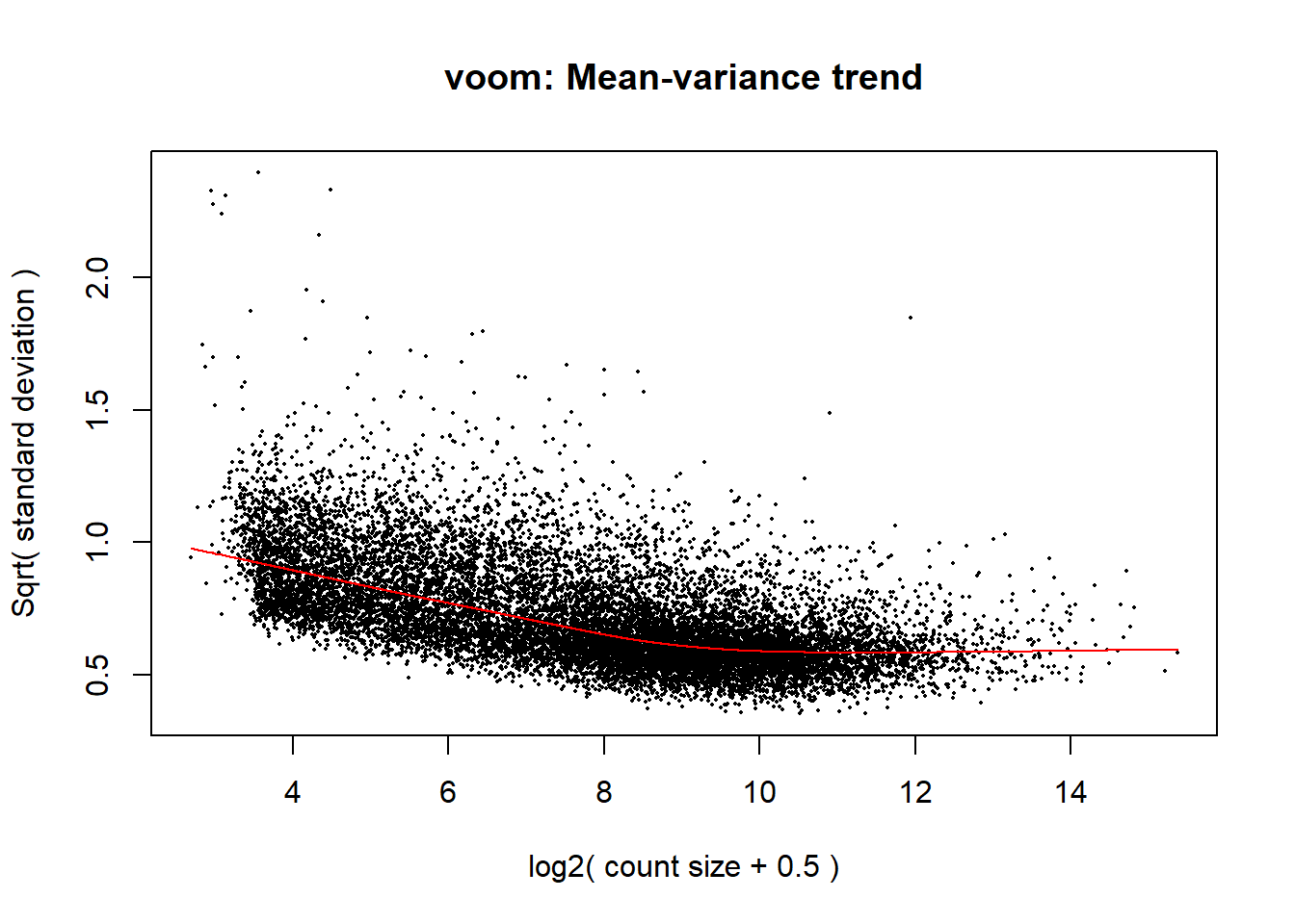
| Version | Author | Date |
|---|---|---|
| 0cb123a | John D. Hurley | 2026-02-18 |
fit <- lmFit(v, design1, block = RNA_Metadata_NoD4_NoRep$Individual, correlation = corfit$consensus.correlation)

contrast_matrix <- makeContrasts(
  HC_D0 = Chimp_Day0 - Human_Day0,
  HC_D2 = Chimp_Day2 - Human_Day2,
  HC_D5 = Chimp_Day5 - Human_Day5,
  HC_D15 = Chimp_Day15 - Human_Day15,
  HC_D30 = Chimp_Day30 - Human_Day30,
  levels = design1)

fit2 <- contrasts.fit(fit,contrast_matrix)
fit2 <- eBayes(fit2)

plotSA(fit2, main = "RNA Model")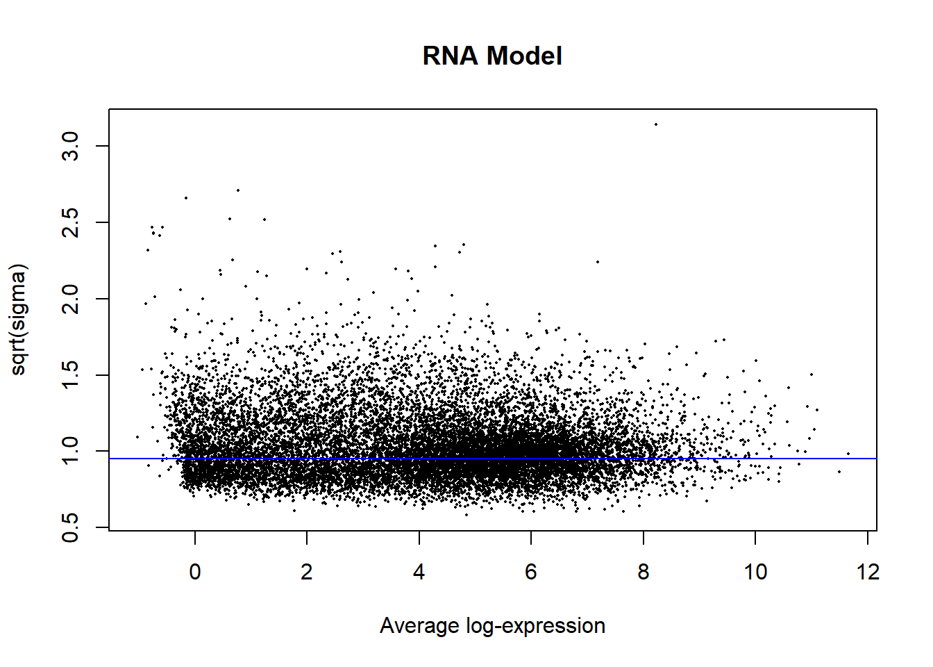
| Version | Author | Date |
|---|---|---|
| 0cb123a | John D. Hurley | 2026-02-18 |
results_summary <- decideTests(fit2,
adjust.method = "BH",
p.value = 0.05)
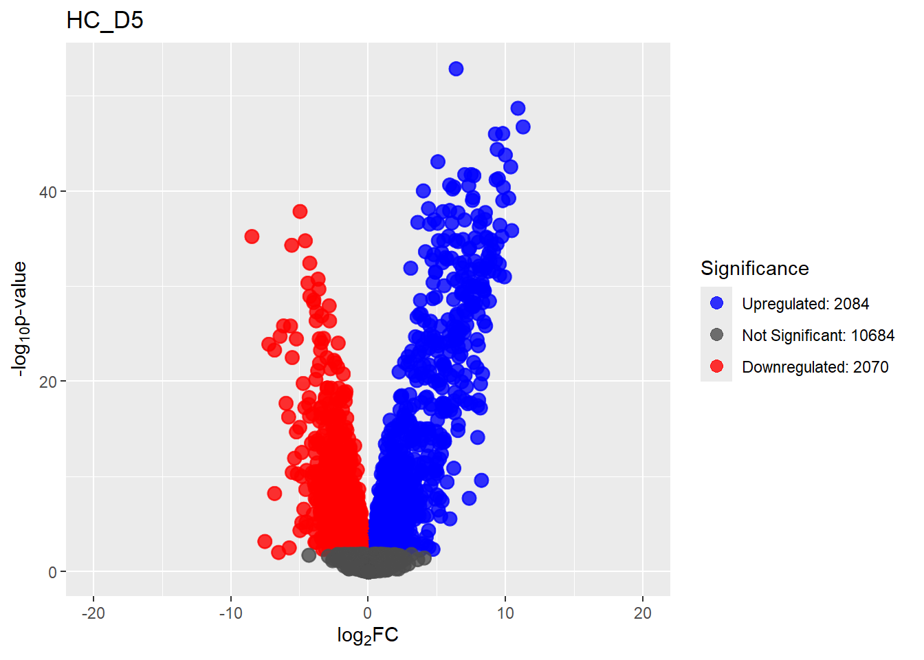
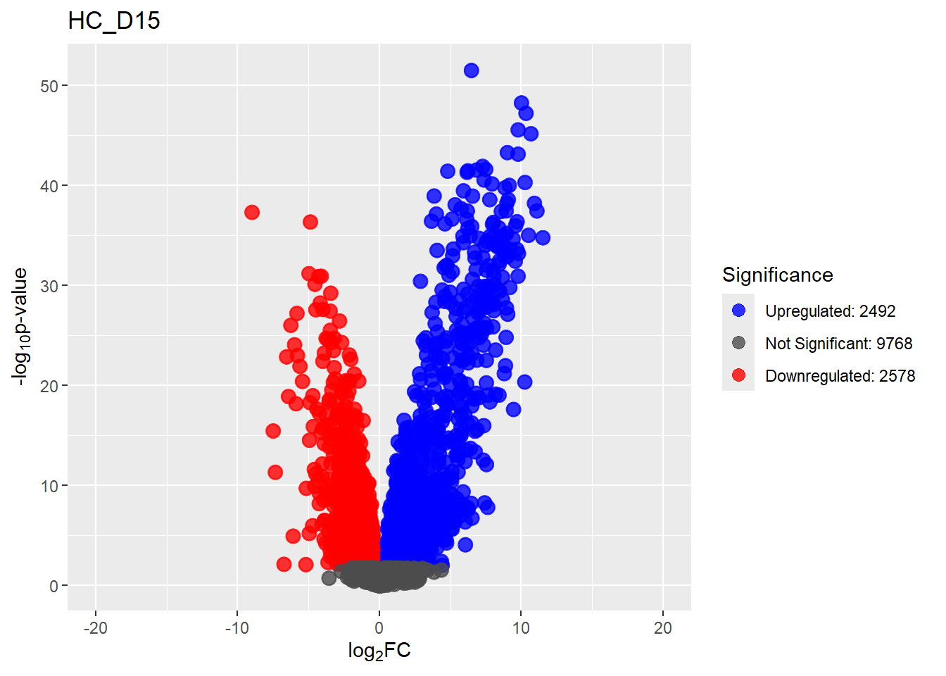
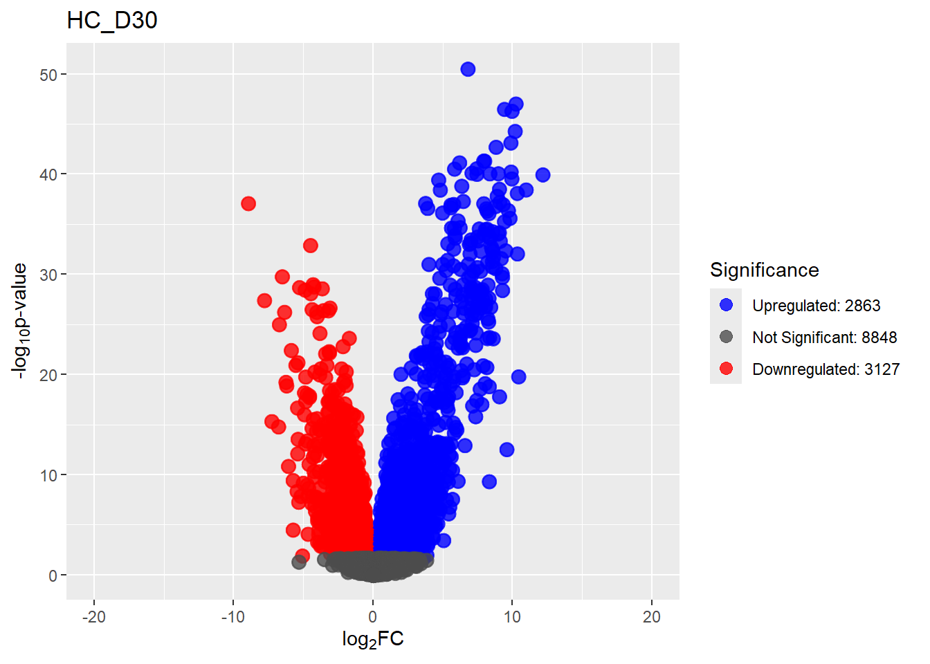
summary(results_summary) HC_D0 HC_D2 HC_D5 HC_D15 HC_D30
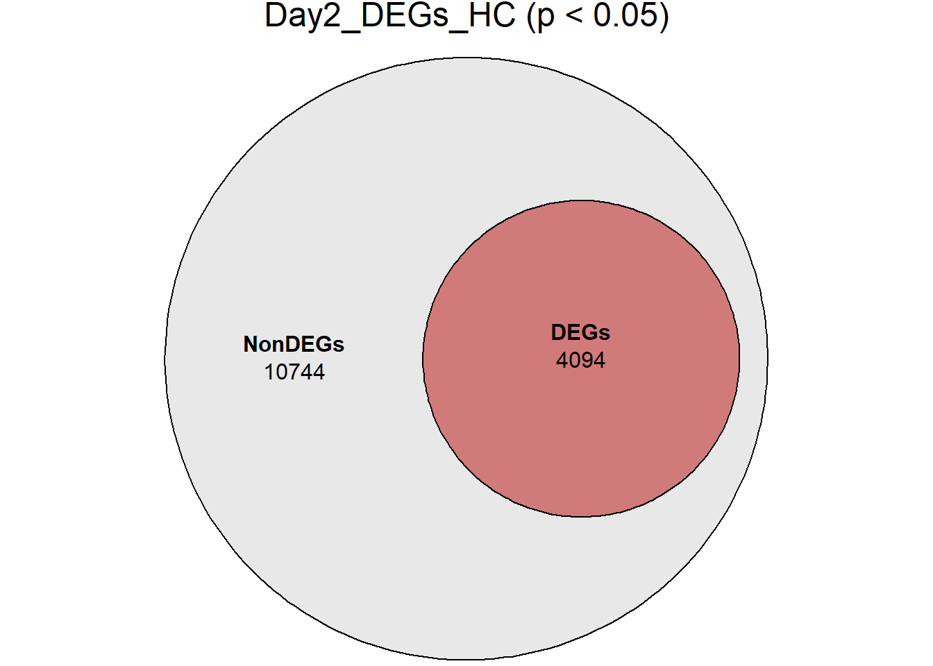
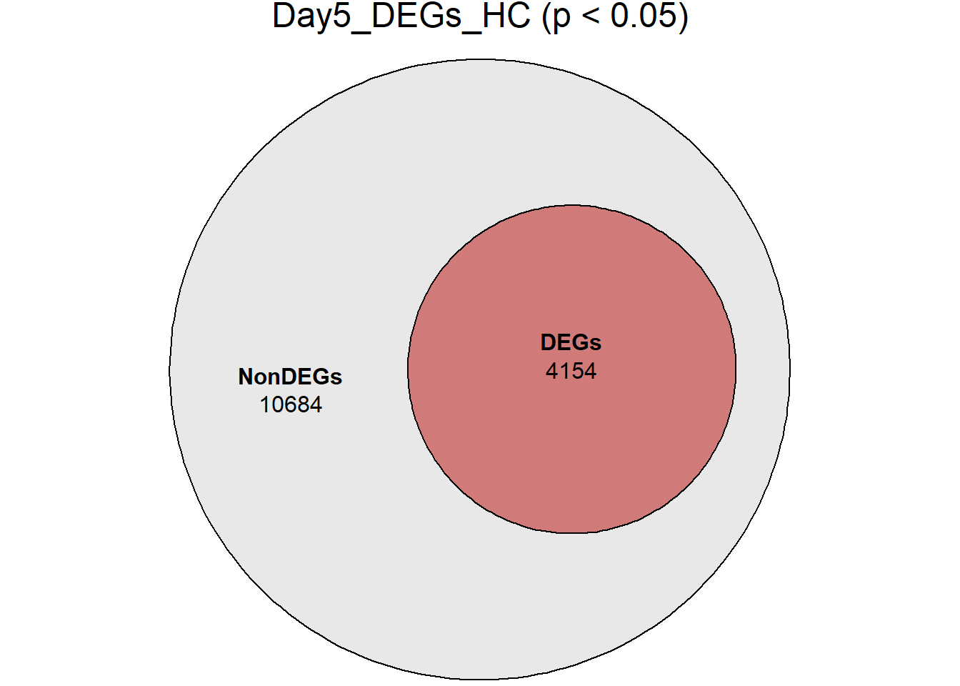
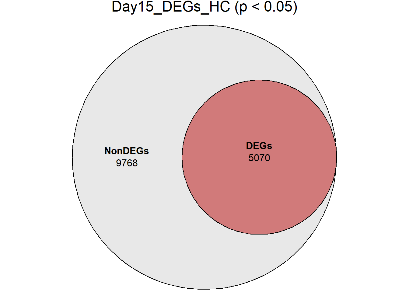
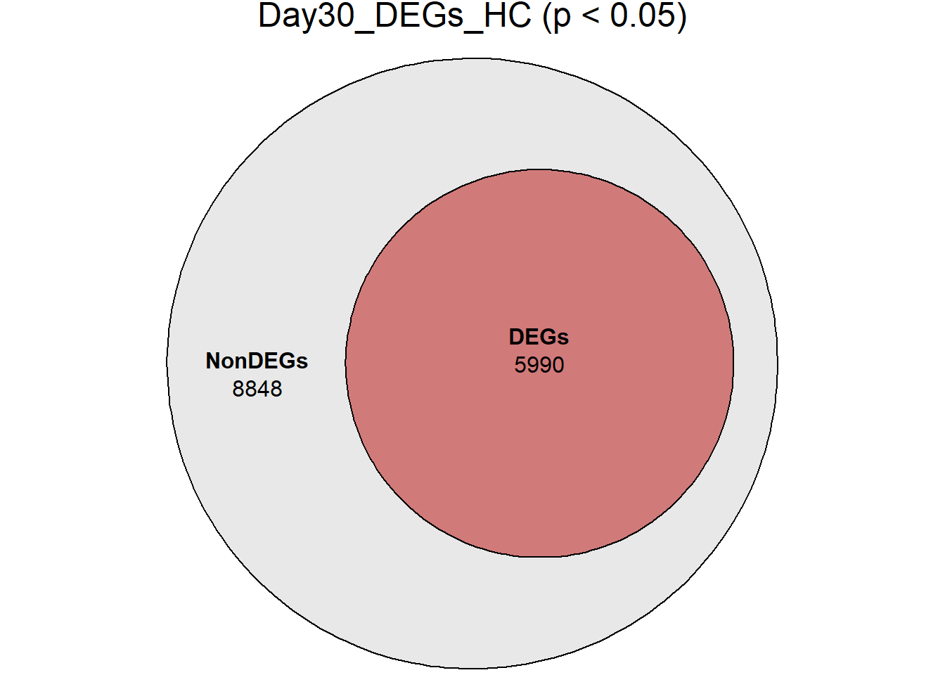
Down 3371 1944 2070 2578 3127
NotSig 8269 10744 10684 9768 8848
Up 3198 2150 2084 2492 2863# saveRDS(fit2,"data/DGE/Species/fit2.RDS")#Create Human TopTable. using listapply, then you can pull specific comp using the $
TopTables_RNA_names <- colnames(fit2$coefficients)
# colnames(fit2$coefficients)
TopTable_RNA_All <- do.call(
rbind,
lapply(TopTables_RNA_names,function(ct) {
tt <- topTable(
fit2,
coef = ct,
number = Inf,
sort.by = "p"
)
#add identifiers
tt$Gene <- rownames(tt)
tt$Comparisons <- ct
tt
})
)
# TopTable_RNA_All$Comparisons
# saveRDS(TopTable_RNA_All,"data/DGE/Species/TopTable_RNA_all.RDS")
head(TopTable_RNA_All) logFC AveExpr t P.Value adj.P.Val
ENSG00000174231 6.604341 5.99612713 52.85392 9.143730e-55 1.356747e-50
ENSG00000184983 11.237428 0.75630938 44.99139 2.230381e-50 1.654720e-46
ENSG00000272540 9.859124 0.05875218 39.97301 3.493933e-47 1.728099e-43
ENSG00000177370 9.890876 0.11451324 39.47648 7.575533e-47 2.252354e-43
ENSG00000231074 10.811687 0.89083894 39.47528 7.589817e-47 2.252354e-43
ENSG00000108953 5.382156 7.03619706 38.02789 7.632500e-46 1.887517e-42
B Gene Comparisons
ENSG00000174231 112.74454 ENSG00000174231 HC_D0
ENSG00000184983 99.69885 ENSG00000184983 HC_D0
ENSG00000272540 93.52547 ENSG00000272540 HC_D0
ENSG00000177370 92.84590 ENSG00000177370 HC_D0
ENSG00000231074 92.94400 ENSG00000231074 HC_D0
ENSG00000108953 94.02074 ENSG00000108953 HC_D0Comparisons_names <- unique(TopTable_RNA_All$Comparisons)
# saveRDS(Comparisons_names,"data/DGE/Species/Comparisons_names_Trajectory.RDS")
plot <- list()
for (n in Comparisons_names) {
plot[[n]] <- TopTable_RNA_All %>%
dplyr::filter(Comparisons == paste0(n)) %>%
generate_volcano_plot(.,n)
}
for (n in Comparisons_names) {
print(plot[[n]])
}
| Version | Author | Date |
|---|---|---|
| b0ab413 | John D. Hurley | 2026-01-28 |
| Version | Author | Date |
|---|---|---|
| b0ab413 | John D. Hurley | 2026-01-28 |
| Version | Author | Date |
|---|---|---|
| b0ab413 | John D. Hurley | 2026-01-28 |
| Version | Author | Date |
|---|---|---|
| b0ab413 | John D. Hurley | 2026-01-28 |
| Version | Author | Date |
|---|---|---|
| b0ab413 | John D. Hurley | 2026-01-28 |
days <- c("D0", "D2", "D5", "D15", "D30")
RNA_sets <- map(
days,
~ {
df <- TopTable_RNA_All %>%
filter(Comparisons == paste0("HC_", .x))
list(
DEGs = df %>% filter(adj.P.Val < 0.05),
NonDEGs = df %>% filter(adj.P.Val >= 0.05)
)
}
)
names(RNA_sets) <- paste0("Day", sub("D", "", days), "_HC")
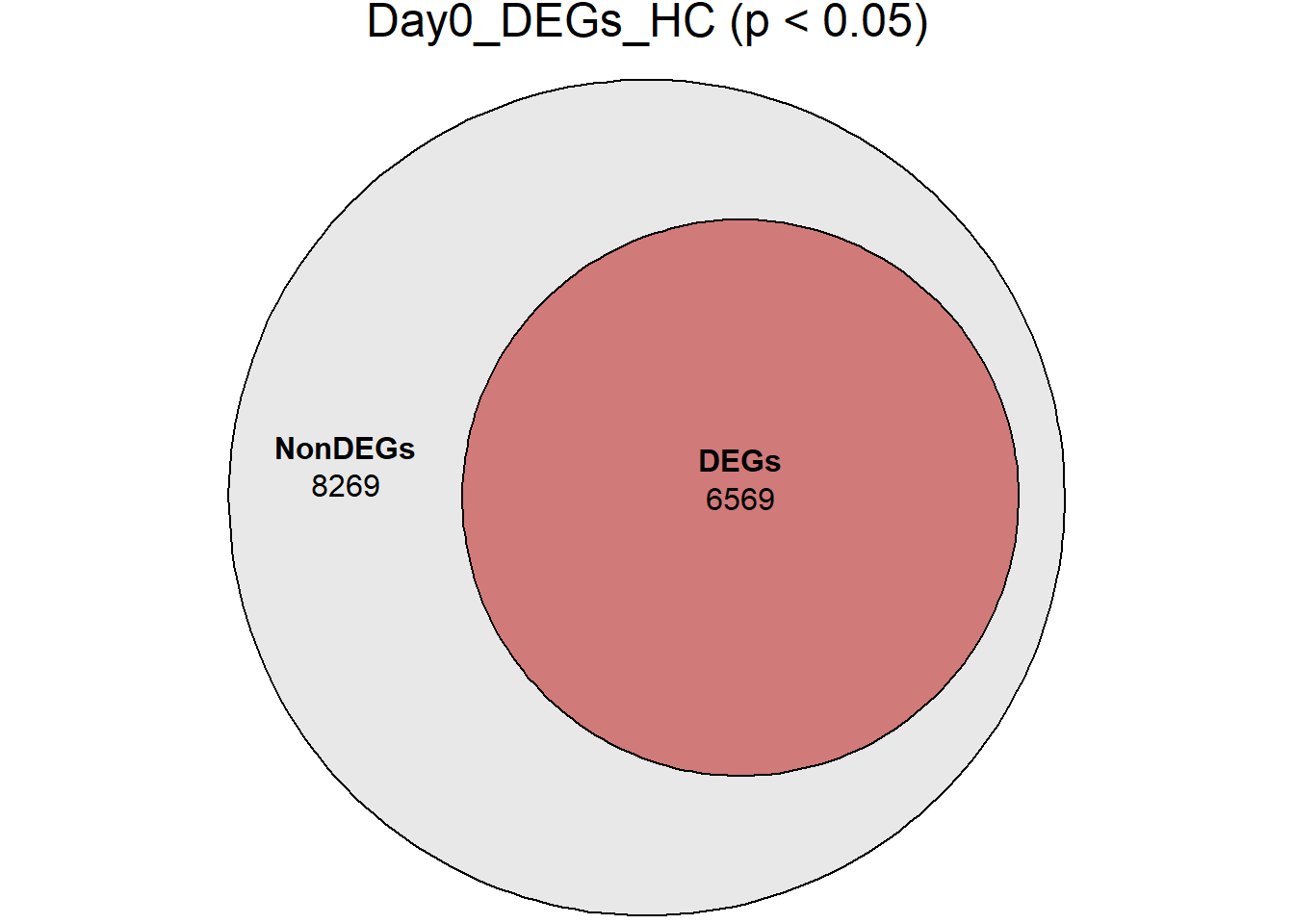
# saveRDS(RNA_sets,"data/DGE/Species/RNA_DEG_Non_DEG_sets_05.RDS")all_genes <- unique(TopTable_RNA_All$Gene)
DEG_Lists <- list(
Day0_DEGs_HC = RNA_sets$Day0_HC$DEGs, # TopTable data.frame
Day2_DEGs_HC = RNA_sets$Day2_HC$DEGs,
Day5_DEGs_HC = RNA_sets$Day5_HC$DEGs,
Day15_DEGs_HC = RNA_sets$Day15_HC$DEGs,
Day30_DEGs_HC = RNA_sets$Day30_HC$DEGs
)
fit_list <- list()
for (name in names(DEG_Lists)) {
# DEG gene vector
deg_vector <- unique(DEG_Lists[[name]]$Gene)
# Euler with containment
fit_list[[name]] <- euler(list(
AllGenes = all_genes,
DEGs = deg_vector
))
# Plot
print(
plot(
fit_list[[name]],
fills = list(
fill = c("grey85", "firebrick"),
alpha = 0.6
),
labels = c("NonDEGs", "DEGs"),
quantities = TRUE,
main = paste0(name, " (p < 0.05)")
)
)
}
| Version | Author | Date |
|---|---|---|
| 0cb123a | John D. Hurley | 2026-02-18 |
| Version | Author | Date |
|---|---|---|
| 0cb123a | John D. Hurley | 2026-02-18 |
| Version | Author | Date |
|---|---|---|
| 0cb123a | John D. Hurley | 2026-02-18 |
| Version | Author | Date |
|---|---|---|
| 0cb123a | John D. Hurley | 2026-02-18 |
| Version | Author | Date |
|---|---|---|
| 0cb123a | John D. Hurley | 2026-02-18 |
####proportion bar plots####
#first factor the timepoints so that they are in the right order
df <- data.frame(
  Day = c("Day0", "Day2", "Day5", "Day15", "Day30"),
  DEGs = c(6569, 4094, 4145, 5070, 5990),
  Non_DEGs = c(8269, 10744, 10684, 9768, 8848)
)

# Convert to long format for ggplot
df_long <- df %>%
  pivot_longer(cols = c(DEGs, Non_DEGs),
               names_to = "Type",
               values_to = "Count") %>%
  group_by(Day) %>%
  mutate(Proportion = Count / sum(Count))  # calculate proportions

df_long$Day <- factor(df_long$Day,levels = c("Day0", "Day2", "Day5", "Day15", "Day30"),ordered = TRUE)

# df_long

ggplot(df_long, aes(x = Day, y = Proportion, fill = Type)) +
  geom_bar(stat = "identity") +
  scale_y_continuous(labels = scales::percent_format()) +  # show % on y-axis
  scale_fill_manual(values = c("DEGs" = "#E41A1C", "Non_DEGs" = "#377EB8")) + # custom colors
  labs(y = "Proportion", x = "", fill = "",title = "Proportion of Species DEGs p < 0.05") +
  theme_minimal(base_size = 14)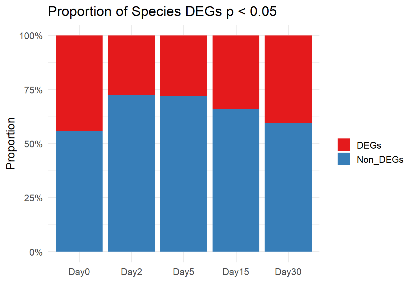
| Version | Author | Date |
|---|---|---|
| 0cb123a | John D. Hurley | 2026-02-18 |
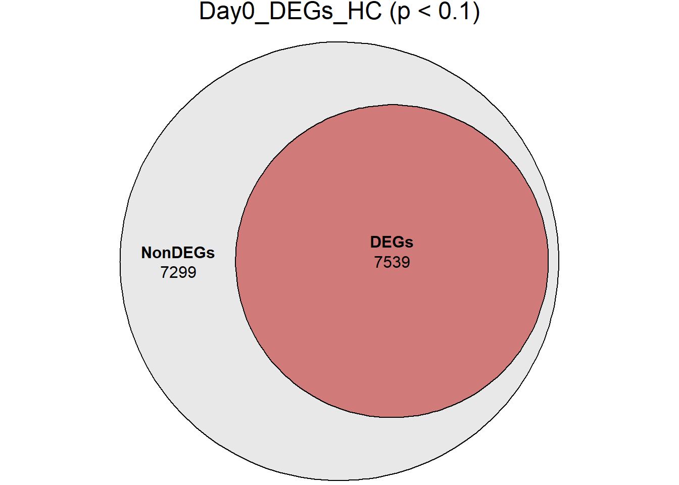
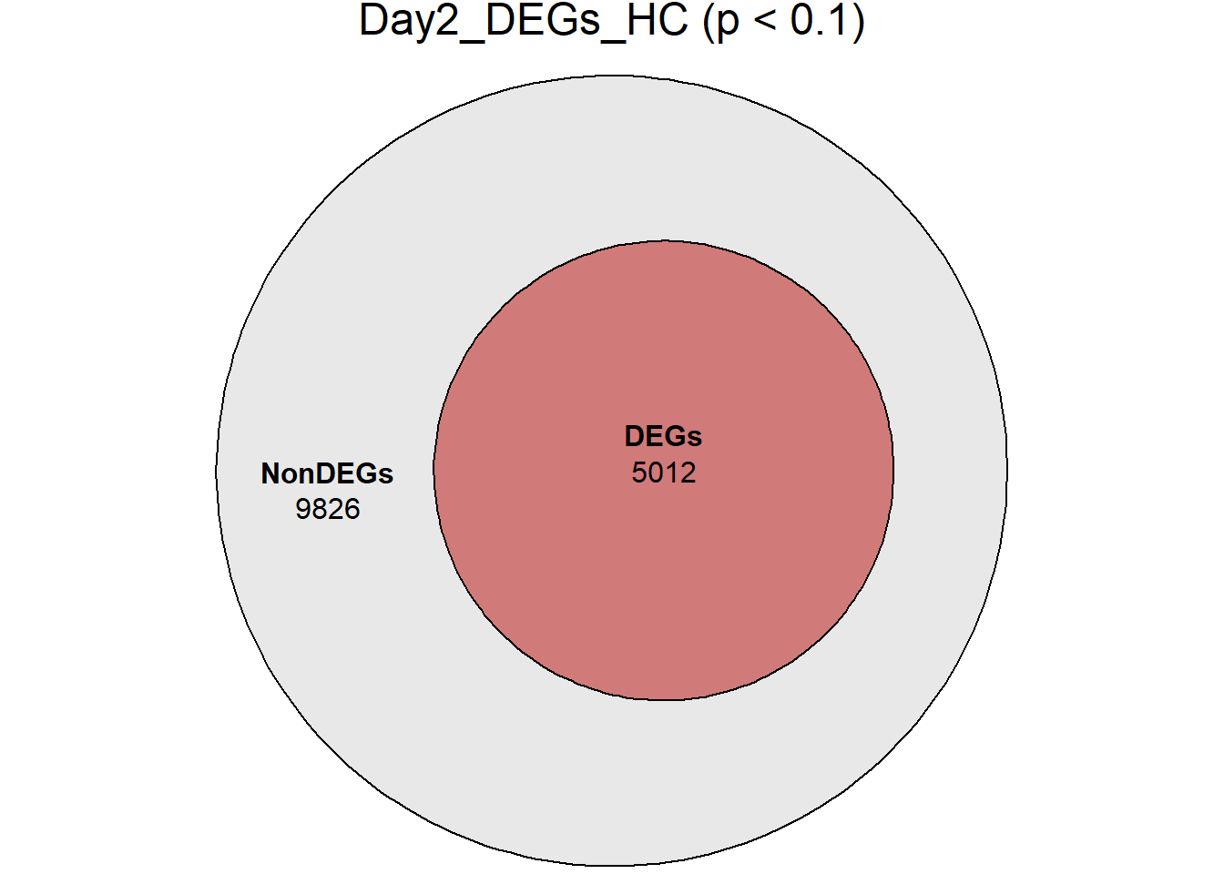
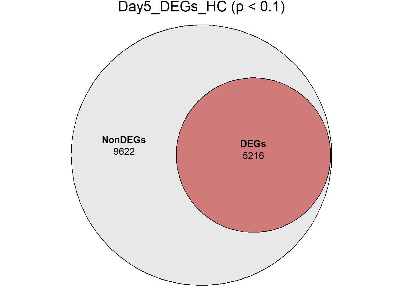
days <- c("D0", "D2", "D5", "D15", "D30")

RNA_sets_0.1 <- map(
  days,
  ~ {
    df <- TopTable_RNA_All %>%
      filter(Comparisons == paste0("HC_", .x))

    list(
      DEGs = df %>% filter(adj.P.Val < 0.1),
      NonDEGs = df %>% filter(adj.P.Val >= 0.1)
    )
  }
)

names(RNA_sets_0.1) <- paste0("Day", sub("D", "", days), "_HC")

# saveRDS(RNA_sets_0.1,"data/DGE/Species/RNA_DEG_Non_DEG_sets_05.RDS")
all_genes <- unique(TopTable_RNA_All$Gene)
DEG_Lists <- list(
Day0_DEGs_HC = RNA_sets_0.1$Day0_HC$DEGs, # TopTable data.frame
Day2_DEGs_HC = RNA_sets_0.1$Day2_HC$DEGs,
Day5_DEGs_HC = RNA_sets_0.1$Day5_HC$DEGs,
Day15_DEGs_HC = RNA_sets_0.1$Day15_HC$DEGs,
Day30_DEGs_HC = RNA_sets_0.1$Day30_HC$DEGs
)
fit_list <- list()
for (name in names(DEG_Lists)) {
# DEG gene vector
deg_vector <- unique(DEG_Lists[[name]]$Gene)
# Euler with containment
fit_list[[name]] <- euler(list(
AllGenes = all_genes,
DEGs = deg_vector
))
# Plot
print(
plot(
fit_list[[name]],
fills = list(
fill = c("grey85", "firebrick"),
alpha = 0.6
),
labels = c("NonDEGs", "DEGs"),
quantities = TRUE,
main = paste0(name, " (p < 0.1)")
)
)
}
| Version | Author | Date |
|---|---|---|
| 0cb123a | John D. Hurley | 2026-02-18 |
| Version | Author | Date |
|---|---|---|
| 0cb123a | John D. Hurley | 2026-02-18 |
| Version | Author | Date |
|---|---|---|
| 0cb123a | John D. Hurley | 2026-02-18 |
| Version | Author | Date |
|---|---|---|
| 0cb123a | John D. Hurley | 2026-02-18 |
| Version | Author | Date |
|---|---|---|
| 0cb123a | John D. Hurley | 2026-02-18 |
####proportion bar plots####
#first factor the timepoints so that they are in the right order
df <- data.frame(
Day = c("Day0", "Day2", "Day5", "Day15", "Day30"),
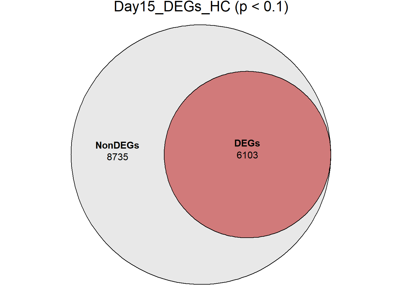
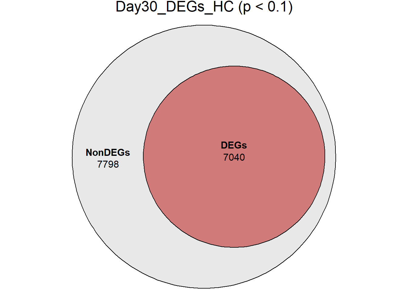
DEGs = c(7539, 5012, 5216, 6103, 7040),
Non_DEGs = c(7299, 9826, 9622, 8735, 7798)
)
# Convert to long format for ggplot
df_long <- df %>%
pivot_longer(cols = c(DEGs, Non_DEGs),
names_to = "Type",
values_to = "Count") %>%
group_by(Day) %>%
mutate(Proportion = Count / sum(Count)) # calculate proportions
df_long$Day <- factor(df_long$Day,levels = c("Day0", "Day2", "Day5", "Day15", "Day30"),ordered = TRUE)
# df_long
ggplot(df_long, aes(x = Day, y = Proportion, fill = Type)) +
geom_bar(stat = "identity") +
scale_y_continuous(labels = scales::percent_format()) + # show % on y-axis
scale_fill_manual(values = c("DEGs" = "#E41A1C", "Non_DEGs" = "#377EB8")) + # custom colors
labs(y = "Proportion", x = "", fill = "", title = "Proportion of Species DEGs p < 0.1") +
theme_minimal(base_size = 14)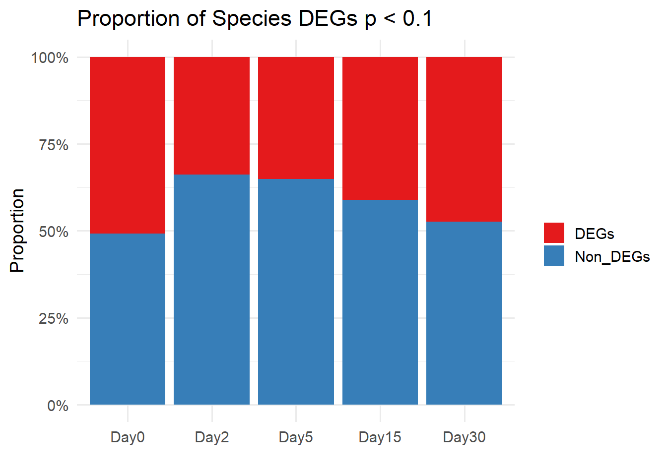
| Version | Author | Date |
|---|---|---|
| 0cb123a | John D. Hurley | 2026-02-18 |
Gene_list <- list(
All_genes = all_genes,
DEGs = deg_genes
)
cluster_plots <- lapply(names(Gene_list), function(clust_name) {
plot_cluster_fc_sig(Gene_list[[clust_name]], clust_name, TopTable_RNA_All)
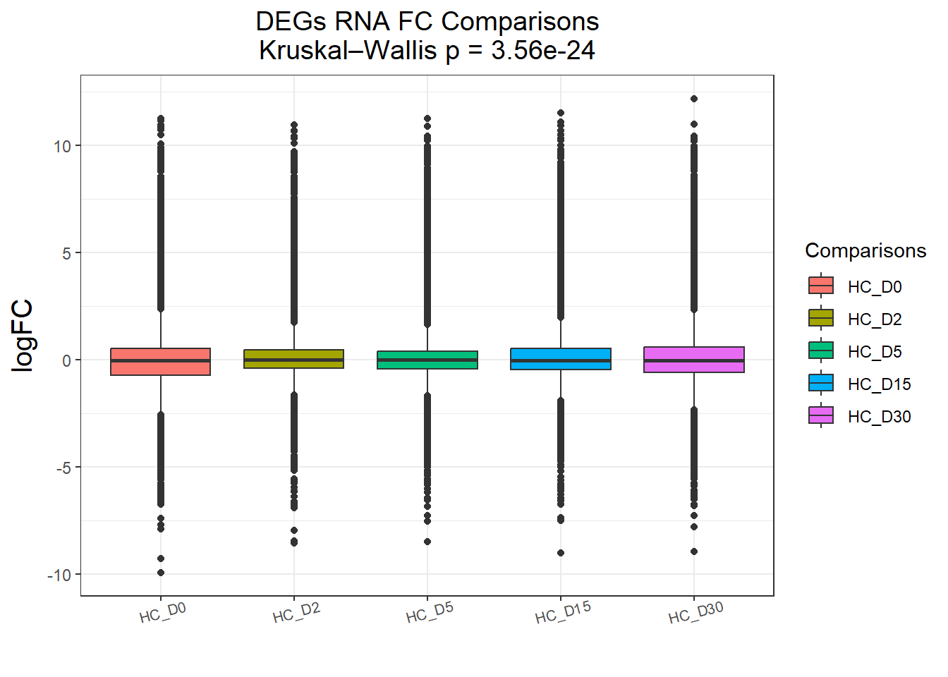
})All_genes : 74190 rows, 14838 unique genes
Pairwise comparisons using Wilcoxon rank sum test with continuity correction
data: df$logFC and df$Comparisons
HC_D0 HC_D2 HC_D5 HC_D15
HC_D2 < 2e-16 - - -
HC_D5 2.8e-10 0.00025 - -
HC_D15 3.7e-13 2.1e-05 0.61867 -
HC_D30 2.7e-08 1.0e-08 0.06482 0.03293
P value adjustment method: BH
DEGs : 58240 rows, 11648 unique genes
Pairwise comparisons using Wilcoxon rank sum test with continuity correction
data: df$logFC and df$Comparisons
HC_D0 HC_D2 HC_D5 HC_D15
HC_D2 < 2e-16 - - -
HC_D5 1.2e-09 0.00561 - -
HC_D15 < 2e-16 0.06704 0.26136 -
HC_D30 2.6e-11 0.00063 0.73944 0.03392
P value adjustment method: BH names(cluster_plots) <- names(Gene_list)
for (p in cluster_plots) print(p)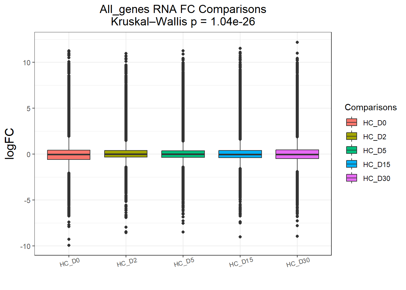
| Version | Author | Date |
|---|---|---|
| 0cb123a | John D. Hurley | 2026-02-18 |
| Version | Author | Date |
|---|---|---|
| 0cb123a | John D. Hurley | 2026-02-18 |
for (comp in Comparisons_names) {

  subset_df <- TopTable_RNA_All %>%
    dplyr::filter(Comparisons == comp)

  cat("\n", comp, "Average logFC:\n")
  cat(mean(subset_df$logFC, na.rm = TRUE), "\n")
}
HC_D0 Average logFC:
-0.04176301
HC_D2 Average logFC:
0.1291112
HC_D5 Average logFC:
0.06418101
HC_D15 Average logFC:
0.1353744
HC_D30 Average logFC:
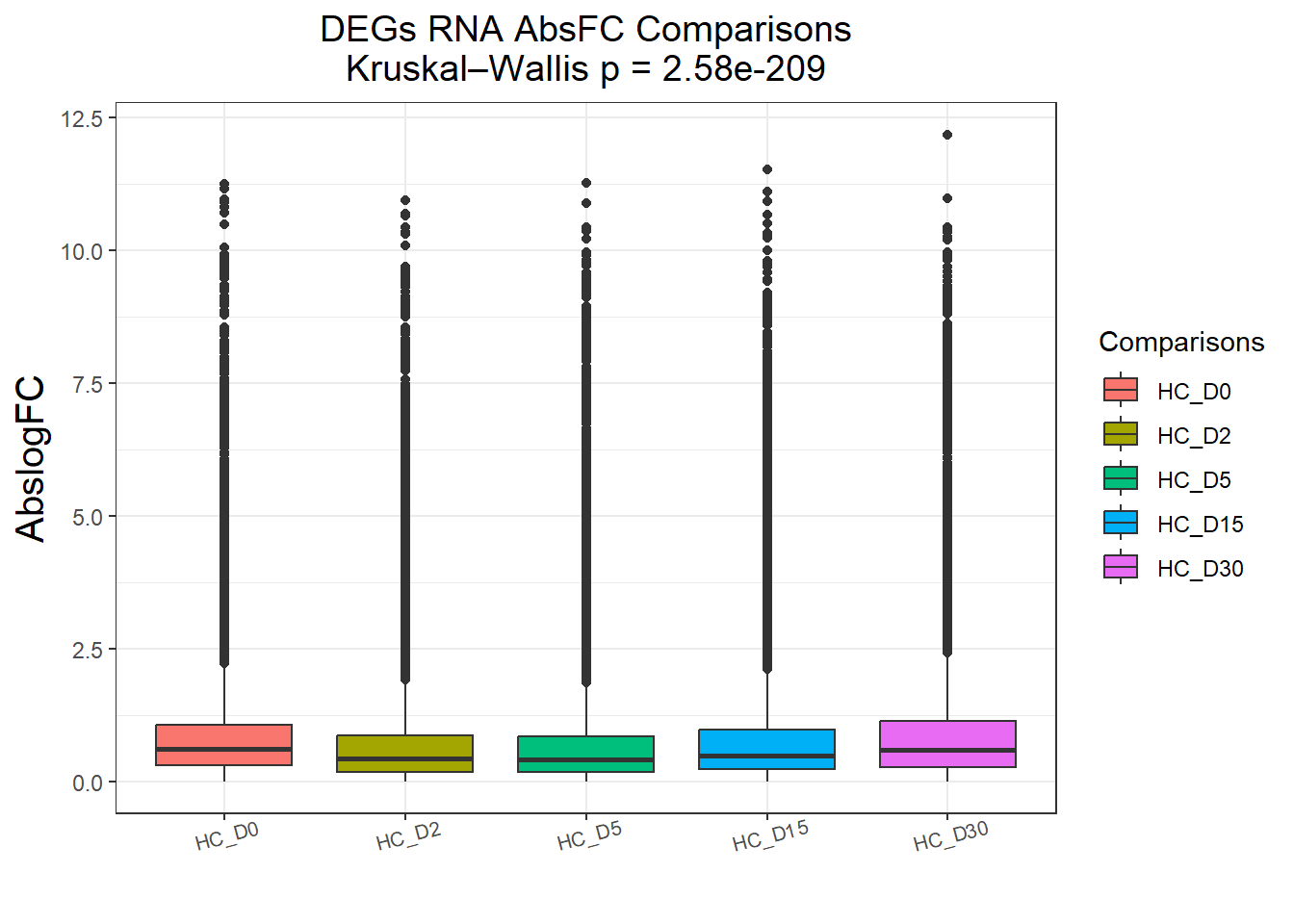
0.10031 all_genes <- readRDS("data/DGE/Species/ExpressedGenes.RDS")
deg_genes <- readRDS("data/DGE/Species/DEG_AtLeastOne.RDS")
TopTable_RNA_All$AbsFC <- abs(TopTable_RNA_All$logFC)
Gene_list <- list(
All_genes = all_genes,
DEGs = deg_genes
)
cluster_plots <- lapply(names(Gene_list), function(clust_name) {
plot_cluster_absfc_sig(Gene_list[[clust_name]], clust_name, TopTable_RNA_All)
})All_genes : 74190 rows, 14838 unique genes
Pairwise comparisons using Wilcoxon rank sum test with continuity correction
data: df$AbsFC and df$Comparisons
HC_D0 HC_D2 HC_D5 HC_D15
HC_D2 < 2e-16 - - -
HC_D5 < 2e-16 0.46 - -
HC_D15 < 2e-16 3.9e-15 < 2e-16 -
HC_D30 0.18 < 2e-16 < 2e-16 < 2e-16
P value adjustment method: BH
DEGs : 58240 rows, 11648 unique genes
Pairwise comparisons using Wilcoxon rank sum test with continuity correction
data: df$AbsFC and df$Comparisons
HC_D0 HC_D2 HC_D5 HC_D15
HC_D2 <2e-16 - - -
HC_D5 <2e-16 0.23 - -
HC_D15 <2e-16 <2e-16 <2e-16 -
HC_D30 0.22 <2e-16 <2e-16 <2e-16
P value adjustment method: BH names(cluster_plots) <- names(Gene_list)
for (p in cluster_plots) print(p)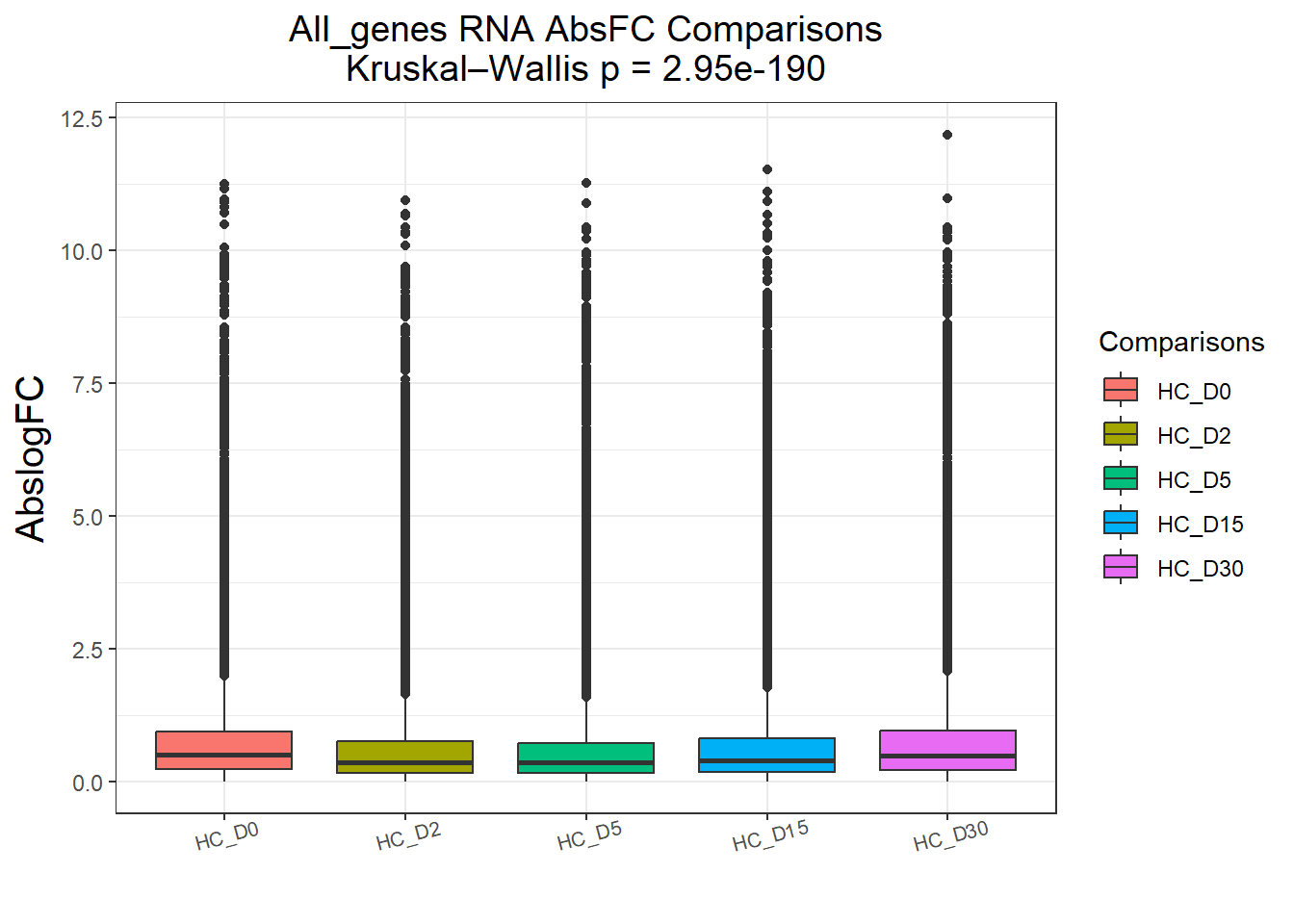
| Version | Author | Date |
|---|---|---|
| 0cb123a | John D. Hurley | 2026-02-18 |
| Version | Author | Date |
|---|---|---|
| 0cb123a | John D. Hurley | 2026-02-18 |
for (comp in Comparisons_names) {

  subset_df <- TopTable_RNA_All %>%
    dplyr::filter(Comparisons == comp)

  cat("\n", comp, "Average AbsFC:\n")
  cat(mean(subset_df$AbsFC, na.rm = TRUE), "\n")
}
 HC_D0 Average AbsFC:
0.7933367

 HC_D2 Average AbsFC:
0.6770691

 HC_D5 Average AbsFC:
0.665505

 HC_D15 Average AbsFC:
0.7349379

 HC_D30 Average AbsFC:
0.8157532
# Your DEGs per day (already defined)
sets <- list(
Day0_DEGs_HC = RNA_sets$Day0_HC$DEGs$Gene, # TopTable data.frame
Day2_DEGs_HC = RNA_sets$Day2_HC$DEGs$Gene,
Day5_DEGs_HC = RNA_sets$Day5_HC$DEGs$Gene,
Day15_DEGs_HC = RNA_sets$Day15_HC$DEGs$Gene,
Day30_DEGs_HC = RNA_sets$Day30_HC$DEGs$Gene
)# Create a 5-way Venn diagram
p <- ggVennDiagram(sets,
label_alpha = 0, # makes background of labels transparent
label = "count") + # show counts in intersections
scale_fill_gradient(low = "skyblue", high = "navy") + # optional color gradient
theme(legend.position = "none") + # hide legend
ggtitle("5-way DEGs")
# Plot
print(p)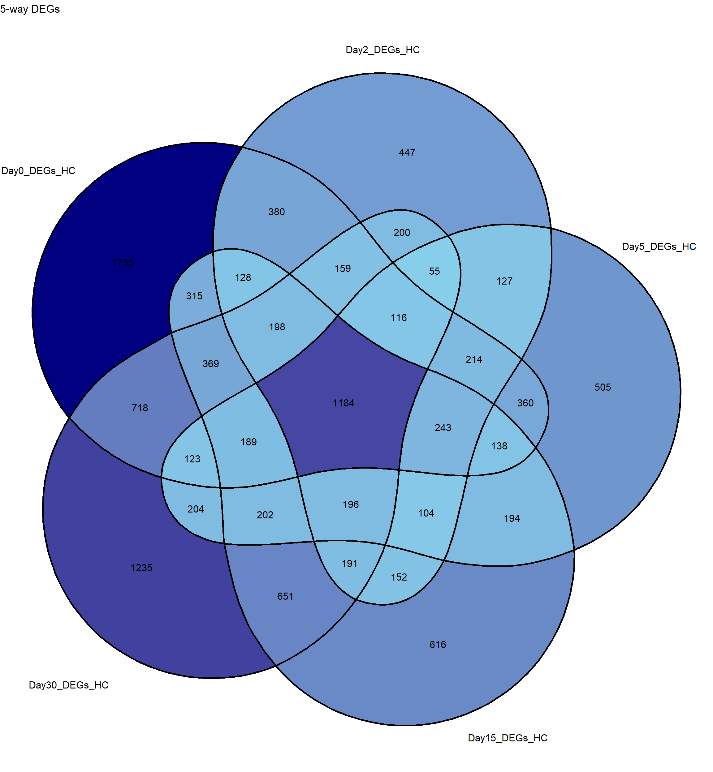
# Helper function to get intersections
get_intersections <- function(sets_list) {
set_names <- names(sets_list)
n <- length(sets_list)
result <- list()
# Loop over all combination lengths (1 to n)
for (k in 1:n) {
combos <- combn(set_names, k, simplify = FALSE)
for (combo in combos) {
# Start with first set in combo
genes <- sets_list[[combo[1]]]
# Intersect with the rest
if (length(combo) > 1) {
for (s in combo[-1]) {
genes <- intersect(genes, sets_list[[s]])
}
}
# Remove genes that appear in other sets outside the combo (exclusive)
other_sets <- setdiff(set_names, combo)
if (length(other_sets) > 0) {
for (s in other_sets) {
genes <- setdiff(genes, sets_list[[s]])
}
}
# Save if any genes remain
if (length(genes) > 0) {
result[[paste(combo, collapse = "&")]] <- genes
}
}
}
return(result)
}
# Compute all intersections
all_intersections <- get_intersections(sets)
# saveRDS(all_intersections,"data/DGE/Species/all_intersections.RDS")
# # Example: genes only in Day0
# all_intersections$Day0
# # Example: genes only in Day0 & Day2
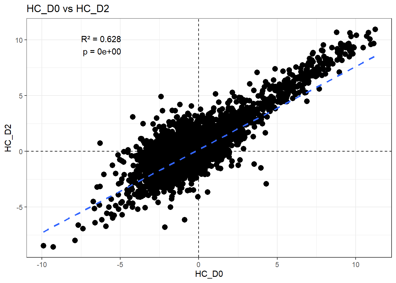
# all_intersections$`Day0&Day2`H_comp <- "HC_D0"
C_comp <- "HC_D2"
df_wide <- TopTable_RNA_All %>%
filter(Comparisons %in% c(H_comp, C_comp)) %>%
dplyr::select(Gene, Comparisons, logFC) %>%
group_by(Gene, Comparisons) %>%
summarize(logFC = mean(logFC), .groups = "drop") %>%
pivot_wider(names_from = Comparisons, values_from = logFC) %>%
filter(!is.na(.data[[H_comp]]), !is.na(.data[[C_comp]]))
# head(df_wide)
# nrow(df_wide)
fit <- lm(df_wide[[C_comp]] ~ df_wide[[H_comp]])
summary(fit)
Call:
lm(formula = df_wide[[C_comp]] ~ df_wide[[H_comp]])

Residuals:
    Min      1Q  Median      3Q     Max
-6.2637 -0.4703 -0.1342  0.3374  6.5623

Coefficients:
                  Estimate Std. Error t value Pr(>|t|)
(Intercept)       0.160214   0.006291   25.47   <2e-16 ***
df_wide[[H_comp]] 0.744745   0.004702  158.41   <2e-16 ***
---
Signif. codes:  0 '***' 0.001 '**' 0.01 '*' 0.05 '.' 0.1 ' ' 1

Residual standard error: 0.7659 on 14836 degrees of freedom
Multiple R-squared:  0.6284,    Adjusted R-squared:  0.6284
F-statistic: 2.509e+04 on 1 and 14836 DF,  p-value: < 2.2e-16
r2 <- summary(fit)$r.squared
pval <- summary(fit)$coefficients[2, "Pr(>|t|)"]
# r2
# pval
# format(pval, scientific = TRUE, digits =3)
x_pos <- max(df_wide[[H_comp]]) * 0.95 # right side
x_neg <- min(df_wide[[H_comp]]) * 0.5 # left side
y_pos <- max(df_wide[[C_comp]]) * 0.95
ggplot(df_wide, aes(x = .data[[H_comp]], y = .data[[C_comp]])) +
geom_point(size = 3) +
geom_smooth(method = "lm", se = FALSE, linetype = "dashed") +
geom_hline(yintercept = 0, linetype = "dashed") +
geom_vline(xintercept = 0, linetype = "dashed") +
annotate(
"text",
x = x_neg,
y = y_pos,
label = paste0(
"R² = ", round(r2, 3),
"\np = ", format(pval, scientific = TRUE, digits = 3)
),
hjust = 1,
vjust = 1
) +
theme_bw() +
labs(
x = H_comp,
y = C_comp,
title = paste0(H_comp, " vs ", C_comp)
)
| Version | Author | Date |
|---|---|---|
| 0cb123a | John D. Hurley | 2026-02-18 |
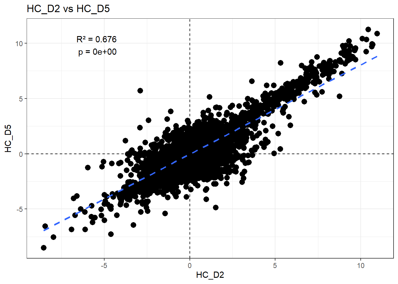
H_comp <- "HC_D2"
C_comp <- "HC_D5"

df_wide <- TopTable_RNA_All %>%
  filter(Comparisons %in% c(H_comp, C_comp)) %>%
  dplyr::select(Gene, Comparisons, logFC) %>%
  group_by(Gene, Comparisons) %>%
  summarize(logFC = mean(logFC), .groups = "drop") %>%
  pivot_wider(names_from = Comparisons, values_from = logFC) %>%
  filter(!is.na(.data[[H_comp]]), !is.na(.data[[C_comp]]))

# head(df_wide)
# nrow(df_wide)

fit <- lm(df_wide[[C_comp]] ~ df_wide[[H_comp]])
summary(fit)
Call:
lm(formula = df_wide[[C_comp]] ~ df_wide[[H_comp]])

Residuals:
    Min      1Q  Median      3Q     Max
-6.0578 -0.2940  0.0238  0.3482  8.1083

Coefficients:
                   Estimate Std. Error t value Pr(>|t|)
(Intercept)       -0.040325   0.005812  -6.938 4.14e-12 ***
df_wide[[H_comp]]  0.809428   0.004602 175.891  < 2e-16 ***
---
Signif. codes:  0 '***' 0.001 '**' 0.01 '*' 0.05 '.' 0.1 ' ' 1

Residual standard error: 0.7043 on 14836 degrees of freedom
Multiple R-squared:  0.6759,    Adjusted R-squared:  0.6759
F-statistic: 3.094e+04 on 1 and 14836 DF,  p-value: < 2.2e-16
r2 <- summary(fit)$r.squared
pval <- summary(fit)$coefficients[2, "Pr(>|t|)"]
# r2
# pval
# format(pval, scientific = TRUE, digits = 3)
library(ggplot2)
x_pos <- max(df_wide[[H_comp]]) * 0.95 # right side
x_neg <- min(df_wide[[H_comp]]) * 0.5 # left side
y_pos <- max(df_wide[[C_comp]]) * 0.95
ggplot(df_wide, aes(x = .data[[H_comp]], y = .data[[C_comp]])) +
geom_point(size = 3) +
geom_smooth(method = "lm", se = FALSE, linetype = "dashed") +
geom_hline(yintercept = 0, linetype = "dashed") +
geom_vline(xintercept = 0, linetype = "dashed") +
annotate(
"text",
x = x_neg,
y = y_pos,
label = paste0(
"R² = ", round(r2, 3),
"\np = ", format(pval, scientific = TRUE, digits = 3)
),
hjust = 1,
vjust = 1
) +
theme_bw() +
labs(
x = H_comp,
y = C_comp,
title = paste0(H_comp, " vs ", C_comp)
)
| Version | Author | Date |
|---|---|---|
| 0cb123a | John D. Hurley | 2026-02-18 |
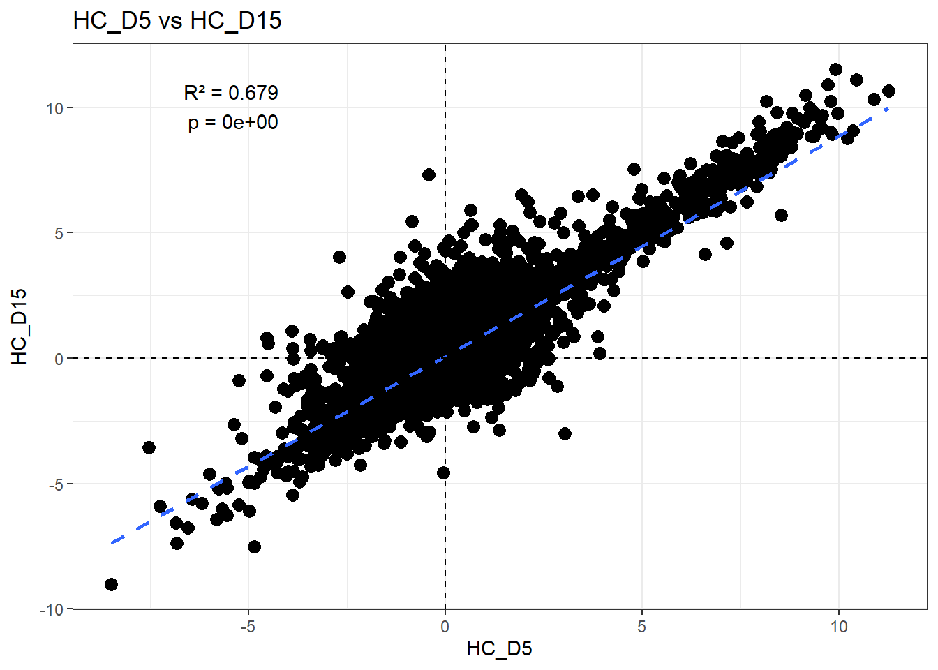
H_comp <- "HC_D5"
C_comp <- "HC_D15"

df_wide <- TopTable_RNA_All %>%
  filter(Comparisons %in% c(H_comp, C_comp)) %>%
  dplyr::select(Gene, Comparisons, logFC) %>%
  group_by(Gene, Comparisons) %>%
  summarize(logFC = mean(logFC), .groups = "drop") %>%
  pivot_wider(names_from = Comparisons, values_from = logFC) %>%
  filter(!is.na(.data[[H_comp]]), !is.na(.data[[C_comp]]))

# head(df_wide)
# nrow(df_wide)

fit <- lm(df_wide[[C_comp]] ~ df_wide[[H_comp]])
summary(fit)
Call:
lm(formula = df_wide[[C_comp]] ~ df_wide[[H_comp]])

Residuals:
    Min      1Q  Median      3Q     Max
-5.7407 -0.4346 -0.0991  0.2863  7.6044

Coefficients:
                  Estimate Std. Error t value Pr(>|t|)
(Intercept)       0.079014   0.006138   12.87   <2e-16 ***
df_wide[[H_comp]] 0.878150   0.004956  177.20   <2e-16 ***
---
Signif. codes:  0 '***' 0.001 '**' 0.01 '*' 0.05 '.' 0.1 ' ' 1

Residual standard error: 0.7467 on 14836 degrees of freedom
Multiple R-squared:  0.6791,    Adjusted R-squared:  0.6791
F-statistic: 3.14e+04 on 1 and 14836 DF,  p-value: < 2.2e-16
r2 <- summary(fit)$r.squared
pval <- summary(fit)$coefficients[2, "Pr(>|t|)"]
# r2
# pval
# format(pval, scientific = TRUE, digits = 3)
x_pos <- max(df_wide[[H_comp]]) * 0.95 # right side
x_neg <- min(df_wide[[H_comp]]) * 0.5 # left side
y_pos <- max(df_wide[[C_comp]]) * 0.95
ggplot(df_wide, aes(x = .data[[H_comp]], y = .data[[C_comp]])) +
geom_point(size = 3) +
geom_smooth(method = "lm", se = FALSE, linetype = "dashed") +
geom_hline(yintercept = 0, linetype = "dashed") +
geom_vline(xintercept = 0, linetype = "dashed") +
annotate(
"text",
x = x_neg,
y = y_pos,
label = paste0(
"R² = ", round(r2, 3),
"\np = ", format(pval, scientific = TRUE, digits = 3)
),
hjust = 1,
vjust = 1
) +
theme_bw() +
labs(
x = H_comp,
y = C_comp,
title = paste0(H_comp, " vs ", C_comp)
)
| Version | Author | Date |
|---|---|---|
| 0cb123a | John D. Hurley | 2026-02-18 |
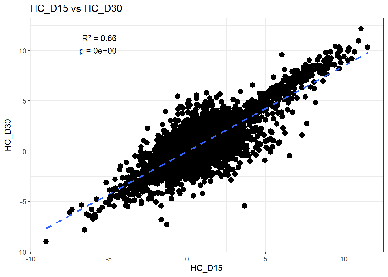
H_comp <- "HC_D15"
C_comp <- "HC_D30"

df_wide <- TopTable_RNA_All %>%
  filter(Comparisons %in% c(H_comp, C_comp)) %>%
  dplyr::select(Gene, Comparisons, logFC) %>%
  group_by(Gene, Comparisons) %>%
  summarize(logFC = mean(logFC), .groups = "drop") %>%
  pivot_wider(names_from = Comparisons, values_from = logFC) %>%
  filter(!is.na(.data[[H_comp]]), !is.na(.data[[C_comp]]))

# head(df_wide)
# nrow(df_wide)

fit <- lm(df_wide[[C_comp]] ~ df_wide[[H_comp]])
summary(fit)
Call:
lm(formula = df_wide[[C_comp]] ~ df_wide[[H_comp]])

Residuals:
    Min      1Q  Median      3Q     Max
-8.5173 -0.3344 -0.0048  0.3363  6.0096

Coefficients:
                   Estimate Std. Error t value Pr(>|t|)
(Intercept)       -0.014621   0.006633  -2.204   0.0275 *
df_wide[[H_comp]]  0.848989   0.005006 169.611   <2e-16 ***
---
Signif. codes:  0 '***' 0.001 '**' 0.01 '*' 0.05 '.' 0.1 ' ' 1

Residual standard error: 0.8037 on 14836 degrees of freedom
Multiple R-squared:  0.6598,    Adjusted R-squared:  0.6597
F-statistic: 2.877e+04 on 1 and 14836 DF,  p-value: < 2.2e-16
r2 <- summary(fit)$r.squared
pval <- summary(fit)$coefficients[2, "Pr(>|t|)"]
# r2
# pval
# format(pval, scientific = TRUE, digits = 3)
x_pos <- max(df_wide[[H_comp]]) * 0.95 # right side
x_neg <- min(df_wide[[H_comp]]) * 0.5 # left side
y_pos <- max(df_wide[[C_comp]]) * 0.95
ggplot(df_wide, aes(x = .data[[H_comp]], y = .data[[C_comp]])) +
geom_point(size = 3) +
geom_smooth(method = "lm", se = FALSE, linetype = "dashed") +
geom_hline(yintercept = 0, linetype = "dashed") +
geom_vline(xintercept = 0, linetype = "dashed") +
annotate(
"text",
x = x_neg,
y = y_pos,
label = paste0(
"R² = ", round(r2, 3),
"\np = ", format(pval, scientific = TRUE, digits = 3)
),
hjust = 1,
vjust = 1
) +
theme_bw() +
labs(
x = H_comp,
y = C_comp,
title = paste0(H_comp, " vs ", C_comp)
)
| Version | Author | Date |
|---|---|---|
| 0cb123a | John D. Hurley | 2026-02-18 |
# git -> commit all changes
# git -> push
# wflow_publish("analysis/RNA_DGE_Comp_Species_Ensemble.Rmd")
sessionInfo()R version 4.5.1 (2025-06-13 ucrt)
Platform: x86_64-w64-mingw32/x64
Running under: Windows 11 x64 (build 26100)
Matrix products: default
LAPACK version 3.12.1
locale:
[1] LC_COLLATE=English_United States.utf8
[2] LC_CTYPE=English_United States.utf8
[3] LC_MONETARY=English_United States.utf8
[4] LC_NUMERIC=C
[5] LC_TIME=English_United States.utf8
time zone: America/Chicago
tzcode source: internal
attached base packages:
[1] stats4 stats graphics grDevices utils datasets methods
[8] base
other attached packages:
[1] ggsignif_0.6.4 edgeR_4.6.3 limma_3.64.3
[4] ggrastr_1.0.2 ggVennDiagram_1.5.7 org.Hs.eg.db_3.21.0
[7] AnnotationDbi_1.70.0 IRanges_2.42.0 S4Vectors_0.46.0
[10] Biobase_2.68.0 BiocGenerics_0.54.1 generics_0.1.4
[13] eulerr_7.0.4 patchwork_1.3.2 ggfortify_0.4.19
[16] ggrepel_0.9.6 readxl_1.4.5 lubridate_1.9.5
[19] forcats_1.0.1 stringr_1.6.0 dplyr_1.1.4
[22] purrr_1.2.1 readr_2.1.6 tidyr_1.3.2
[25] tibble_3.3.1 ggplot2_4.0.2 tidyverse_2.0.0
[28] workflowr_1.7.2
loaded via a namespace (and not attached):
[1] DBI_1.2.3 gridExtra_2.3 rlang_1.1.7
[4] magrittr_2.0.4 git2r_0.36.2 otel_0.2.0
[7] compiler_4.5.1 RSQLite_2.4.5 getPass_0.2-4
[10] mgcv_1.9-4 png_0.1-8 callr_3.7.6
[13] vctrs_0.7.1 polylabelr_1.0.0 pkgconfig_2.0.3
[16] crayon_1.5.3 fastmap_1.2.0 XVector_0.48.0
[19] labeling_0.4.3 promises_1.5.0 rmarkdown_2.30
[22] tzdb_0.5.0 UCSC.utils_1.4.0 ps_1.9.1
[25] ggbeeswarm_0.7.3 bit_4.6.0 xfun_0.56
[28] cachem_1.1.0 GenomeInfoDb_1.44.3 jsonlite_2.0.0
[31] blob_1.3.0 later_1.4.5 R6_2.6.1
[34] bslib_0.10.0 stringi_1.8.7 RColorBrewer_1.1-3
[37] jquerylib_0.1.4 cellranger_1.1.0 Rcpp_1.1.1
[40] knitr_1.51 Matrix_1.7-4 httpuv_1.6.16
[43] splines_4.5.1 timechange_0.4.0 tidyselect_1.2.1
[46] rstudioapi_0.18.0 yaml_2.3.12 processx_3.8.6
[49] lattice_0.22-7 withr_3.0.2 KEGGREST_1.48.1
[52] S7_0.2.1 evaluate_1.0.5 polyclip_1.10-7
[55] Biostrings_2.76.0 pillar_1.11.1 whisker_0.4.1
[58] rprojroot_2.1.1 hms_1.1.4 scales_1.4.0
[61] glue_1.8.0 tools_4.5.1 locfit_1.5-9.12
[64] fs_1.6.6 grid_4.5.1 Cairo_1.7-0
[67] nlme_3.1-168 GenomeInfoDbData_1.2.14 beeswarm_0.4.0
[70] vipor_0.4.7 cli_3.6.5 gtable_0.3.6
[73] sass_0.4.10 digest_0.6.39 farver_2.1.2
[76] memoise_2.0.1 htmltools_0.5.9 lifecycle_1.0.5
[79] httr_1.4.7 statmod_1.5.1 bit64_4.6.0-1