RNA_CorrelationHeatMap

workflowr

• Summary
• Checks
• Past versions

Last updated: 2026-04-02

Checks: 7 0

Knit directory: CrossSpecies_CM_Diff_RNA/

This reproducible R Markdown analysis was created with workflowr (version 1.7.2). The Checks tab describes the reproducibility checks that were applied when the results were created. The Past versions tab lists the development history.

---

R Markdown file: up-to-date

Great! Since the R Markdown file has been committed to the Git repository, you know the exact version of the code that produced these results.

Environment: empty

Great job! The global environment was empty. Objects defined in the global environment can affect the analysis in your R Markdown file in unknown ways. For reproduciblity it’s best to always run the code in an empty environment.

Seed: set.seed(20251129)

The command set.seed(20251129) was run prior to running the code in the R Markdown file. Setting a seed ensures that any results that rely on randomness, e.g. subsampling or permutations, are reproducible.

Session information: recorded

Great job! Recording the operating system, R version, and package versions is critical for reproducibility.

Cache: none

Nice! There were no cached chunks for this analysis, so you can be confident that you successfully produced the results during this run.

File paths: relative

Great job! Using relative paths to the files within your workflowr project makes it easier to run your code on other machines.

Repository version: d95f3cc

Great! You are using Git for version control. Tracking code development and connecting the code version to the results is critical for reproducibility.

The results in this page were generated with repository version d95f3cc. See the Past versions tab to see a history of the changes made to the R Markdown and HTML files.

Note that you need to be careful to ensure that all relevant files for the analysis have been committed to Git prior to generating the results (you can use wflow_publish or wflow_git_commit). workflowr only checks the R Markdown file, but you know if there are other scripts or data files that it depends on. Below is the status of the Git repository when the results were generated:

Ignored files:
    Ignored:    .Rhistory
    Ignored:    .Rproj.user/
    Ignored:    data/

Unstaged changes:
    Modified:   analysis/RNA_PCA_Ensemble.Rmd

Note that any generated files, e.g. HTML, png, CSS, etc., are not included in this status report because it is ok for generated content to have uncommitted changes.

---

These are the previous versions of the repository in which changes were made to the R Markdown (analysis/RNA_CorrelationHeatMap_Ensemble.Rmd) and HTML (docs/RNA_CorrelationHeatMap_Ensemble.html) files. If you’ve configured a remote Git repository (see ?wflow_git_remote), click on the hyperlinks in the table below to view the files as they were in that past version.

File	Version	Author	Date	Message
Rmd	d95f3cc	John D. Hurley	2026-04-02	added R Objects for No Day5
html	0c9c163	John D. Hurley	2026-04-02	Build site.
Rmd	5535f1d	John D. Hurley	2026-04-02	added toptable RObject
Rmd	904e533	John D. Hurley	2026-04-01	naming sections correction 4/1/26
Rmd	68d1adb	John D. Hurley	2026-04-01	webstie update 4/1/26
html	9d3ae04	John D. Hurley	2026-03-30	Build site.
Rmd	5a7c251	John D. Hurley	2026-03-30	Changes to data QC checks
html	0958201	John D. Hurley	2026-03-23	Build site.
Rmd	01611df	John D. Hurley	2026-03-23	Data updates
html	8bce9df	John D. Hurley	2026-02-20	Build site.
html	fcf8fc0	John D. Hurley	2026-02-18	Build site.
Rmd	c85837b	John D. Hurley	2026-02-18	SiteUpDate_CorrelationHeatMap
html	7789dff	John D. Hurley	2026-01-28	Build site.
Rmd	0fcf7c3	John D. Hurley	2026-01-28	HeatMap knit update
html	d9f15a6	John D. Hurley	2026-01-28	Build site.
Rmd	19cd9fb	John D. Hurley	2026-01-28	Commenting out wokrflowr publish
Rmd	3b54f65	John D. Hurley	2026-01-28	Duplicate Code Labels
Rmd	de67e64	John D. Hurley	2026-01-28	Commenting out code not in use.
Rmd	da444ed	John D. Hurley	2026-01-28	RMarkdown name update
Rmd	085c1db	John D. Hurley	2026-01-28	Finalizing CorHeatMap

---

RNA_Metadata <- read_excel("~/diff_timeline_tes/RNA/RNA_Metadata.xlsx")
counts_table <- read.delim("~/diff_timeline_tes/RNA/rna_concat/featureCounts/all_counts.txt")
marker_genes <- read.delim("~/diff_timeline_tes/RNA/CM_Diff_PurityPanel.txt")

RNA_fc <- counts_table %>%
  filter(Geneid != "#") %>%
  filter(Geneid != "Geneid") %>%
  column_to_rownames("Geneid")

# #Rename column Names to More Useful Info
col_names <- RNA_Metadata$SampleName
colnames(RNA_fc) <- col_names
dim(RNA_fc)

ensembl_ids_unfilt <- rownames(RNA_fc)
entrez_ids_unfilt <- mapIds(org.Hs.eg.db,
                            keys = ensembl_ids_unfilt,
                            column = "ENTREZID",
                            keytype = "ENSEMBL",
                            multiVals = "first")
symbol_ids_unfilt <- mapIds(org.Hs.eg.db,
                            keys = ensembl_ids_unfilt,
                            column = "SYMBOL",
                            keytype = "ENSEMBL",
                            multiVals = "first")

RNA_fc_df <- as.data.frame(RNA_fc)
RNA_fc_df <- RNA_fc_df %>%
  rownames_to_column(var = "Ensemble") %>%
  dplyr::mutate(
    Entrez_ID = entrez_ids_unfilt,
    Symbol    = symbol_ids_unfilt
  ) %>%
  dplyr::select(
    Ensemble,        # 1st column
    Entrez_ID,       # 2nd column
    Symbol,          # 3rd column
    everything()     # rest unchanged
  )

rn <- rownames(RNA_fc)

RNA_fc <- as.data.frame(
  lapply(RNA_fc, function(x) as.numeric(as.character(x)))
)

rownames(RNA_fc) <- rn

# saveRDS(RNA_fc,"data/QC/concat/RNA_fc.RDS")
# saveRDS(RNA_fc_df,"data/Raw_Data/concat/RNA_fc_df.RDS")
# saveRDS(RNA_Metadata,"data/Raw_Data/concat/RNA_Metadata.RDS")
# saveRDS(marker_genes,"data/Raw_Data/concat/marker_genes.RDS")

total_reads_df <- RNA_fc %>%
  as.data.frame() %>%
  mutate(Gene = rownames(.)) %>%
  dplyr::select(-Gene) %>%
  summarise(across(everything(), \(x) sum(x, na.rm = TRUE))) %>%
  pivot_longer(
    cols = everything(),
    names_to = "Sample",
    values_to = "Total_Counts"
  ) %>%
  left_join(RNA_Metadata, by = c("Sample" = "SampleName"))

day_levels <- c("Day0","Day2","Day4","Day5","Day15","Day30")

total_reads_df <- total_reads_df %>%
  mutate(
    Timepoint = factor(Timepoint, levels = day_levels, ordered = TRUE),

    # force species order: chimp first, human second
    Species = factor(Species, levels = c("C", "H")),

    Individual_Color = ann_colors$individual_cor[Individual]
  ) %>%
  arrange(Species, Individual, Timepoint) %>%
  mutate(Sample = factor(Sample, levels = Sample))

library(ggplot2)

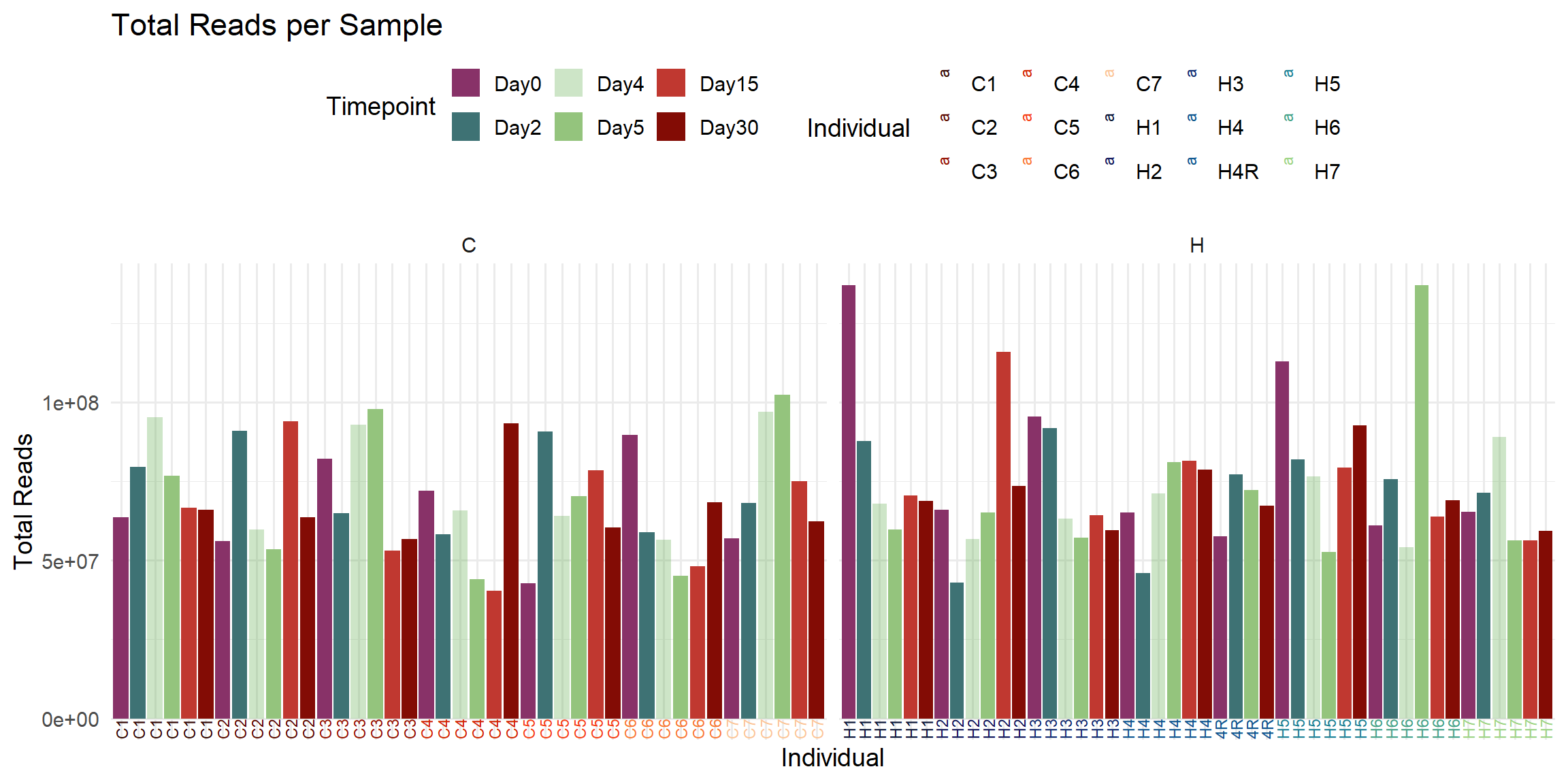
ggplot(total_reads_df, aes(x = Sample, y = Total_Reads, fill = Timepoint)) +
  geom_col() +
  geom_text(aes(label = Individual, color = Individual), 
            y = 0, angle = 90, hjust = 1, vjust = 0.5, size = 3) +
  scale_fill_manual(values = ann_colors$timepoint_cor) +
  scale_color_manual(values = ann_colors$individual_cor) +
  facet_wrap(~Species, scales = "free_x") +
  theme_minimal(base_size = 14) +
  theme(axis.text.x = element_blank(),
        axis.ticks.x = element_blank(),
        legend.position = "top") +
  labs(
    title = "Total Reads per Sample",
    x = "Individual",
    y = "Total Reads",
    fill = "Timepoint",
    color = "Individual"
  )

Past versions of RNASeq_perSample_graph-1.png

Version	Author	Date
0c9c163	John D. Hurley	2026-04-02

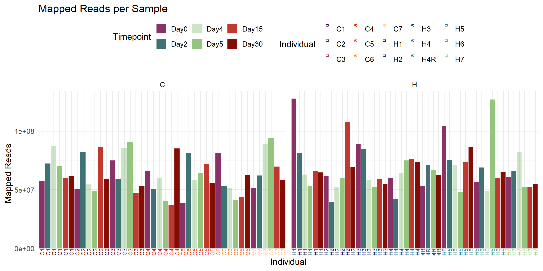
ggplot(total_reads_df, aes(x = Sample, y = Mapped_Reads, fill = Timepoint)) +
  geom_col() +
  geom_text(aes(label = Individual, color = Individual), 
            y = 0, angle = 90, hjust = 1, vjust = 0.5, size = 3) +
  scale_fill_manual(values = ann_colors$timepoint_cor) +
  scale_color_manual(values = ann_colors$individual_cor) +
  facet_wrap(~Species, scales = "free_x") +
  theme_minimal(base_size = 14) +
  theme(axis.text.x = element_blank(),
        axis.ticks.x = element_blank(),
        legend.position = "top") +
  labs(
    title = "Mapped Reads per Sample",
    x = "Individual",
    y = "Mapped Reads",
    fill = "Timepoint",
    color = "Individual"
  )

Past versions of RNASeq_perSample_graph-2.png

Version	Author	Date
0c9c163	John D. Hurley	2026-04-02

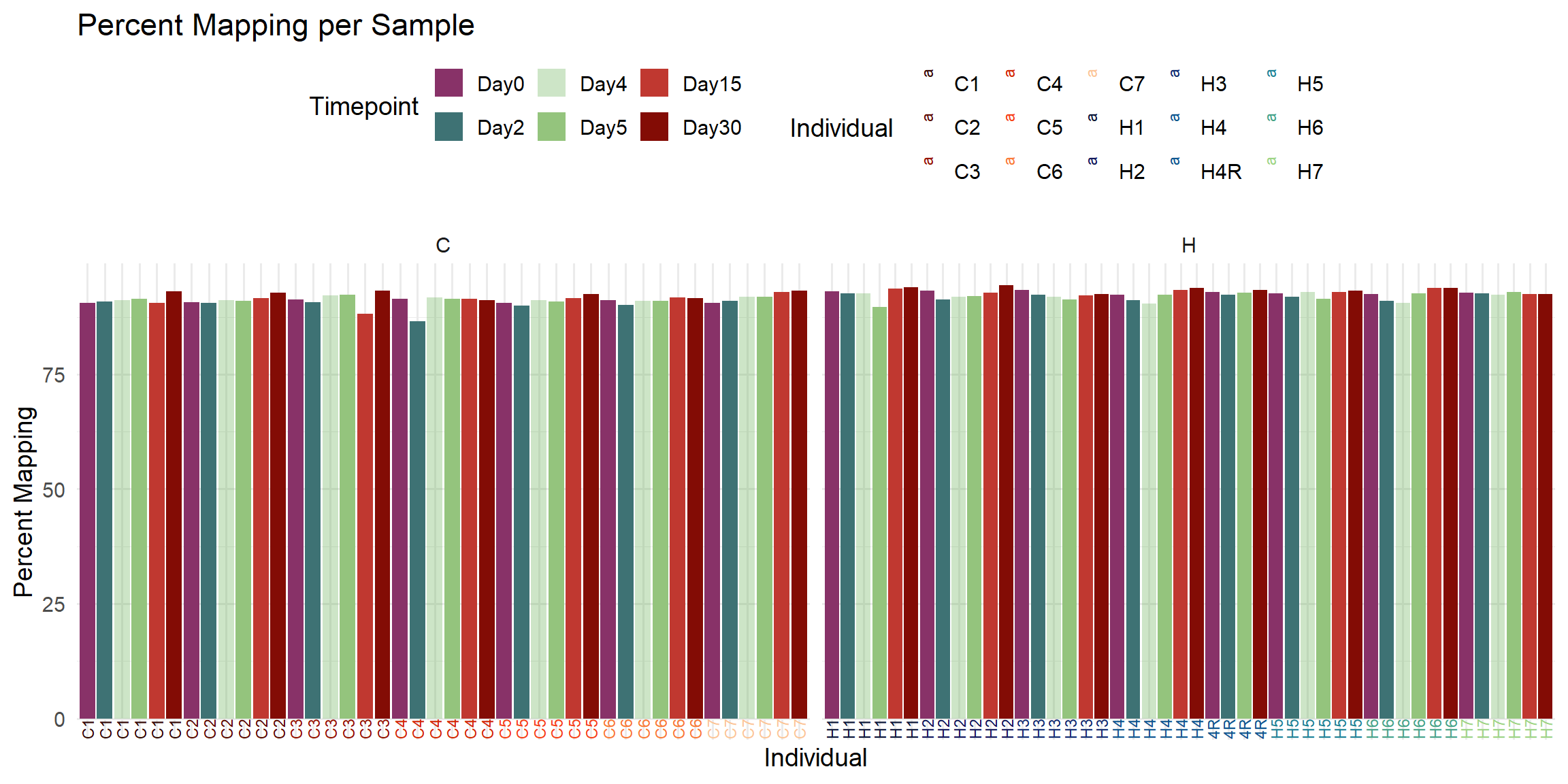
ggplot(total_reads_df, aes(x = Sample, y = Percent_Mapped, fill = Timepoint)) +
  geom_col() +
  geom_text(aes(label = Individual, color = Individual), 
            y = 0, angle = 90, hjust = 1, vjust = 0.5, size = 3) +
  scale_fill_manual(values = ann_colors$timepoint_cor) +
  scale_color_manual(values = ann_colors$individual_cor) +
  facet_wrap(~Species, scales = "free_x") +
  theme_minimal(base_size = 14) +
  theme(axis.text.x = element_blank(),
        axis.ticks.x = element_blank(),
        legend.position = "top") +
  labs(
    title = "Percent Mapping per Sample",
    x = "Individual",
    y = "Percent Mapping",
    fill = "Timepoint",
    color = "Individual"
  )

Past versions of RNASeq_perSample_graph-3.png

Version	Author	Date
0c9c163	John D. Hurley	2026-04-02

ggplot(total_reads_df, aes(x = Sample, y = Usable_Fragments, fill = Timepoint)) +
  geom_col() +
  geom_text(aes(label = Individual, color = Individual), 
            y = 0, angle = 90, hjust = 1, vjust = 0.5, size = 3) +
  scale_fill_manual(values = ann_colors$timepoint_cor) +
  scale_color_manual(values = ann_colors$individual_cor) +
  facet_wrap(~Species, scales = "free_x") +
  theme_minimal(base_size = 14) +
  theme(axis.text.x = element_blank(),
        axis.ticks.x = element_blank(),
        legend.position = "top") +
  labs(
    title = "Usable Fragments per Sample",
    x = "Individual",
    y = "Number Fragments",
    fill = "Timepoint",
    color = "Individual"
  )

Past versions of RNASeq_perSample_graph-4.png

Version	Author	Date
0c9c163	John D. Hurley	2026-04-02

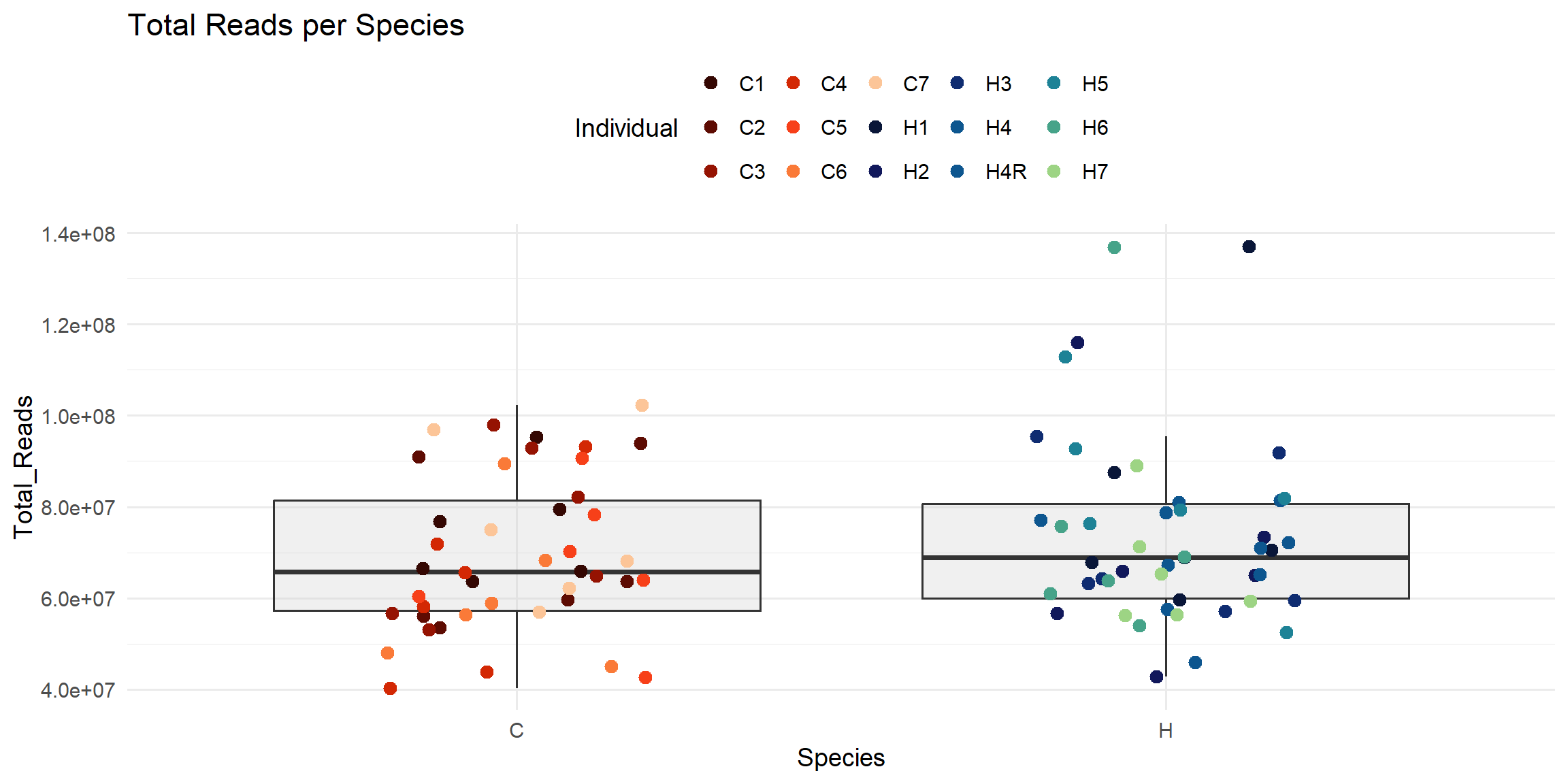
ggplot(total_reads_df, aes(x = Species, y = Total_Reads)) +
  geom_boxplot(fill = "#CCCCCC", alpha = 0.3, outlier.shape = NA) +
  geom_jitter(aes(color = Individual), width = 0.2, size = 3) +
  scale_color_manual(values = ann_colors$individual_cor) +
  theme_minimal(base_size = 14) +
  theme(legend.position = "top") +
  labs(
    title = "Total Reads per Species",
    x = "Species",
    y = "Total_Reads",
    color = "Individual"
  )

Past versions of RNASeq_perSpecies_graph-1.png

Version	Author	Date
0c9c163	John D. Hurley	2026-04-02

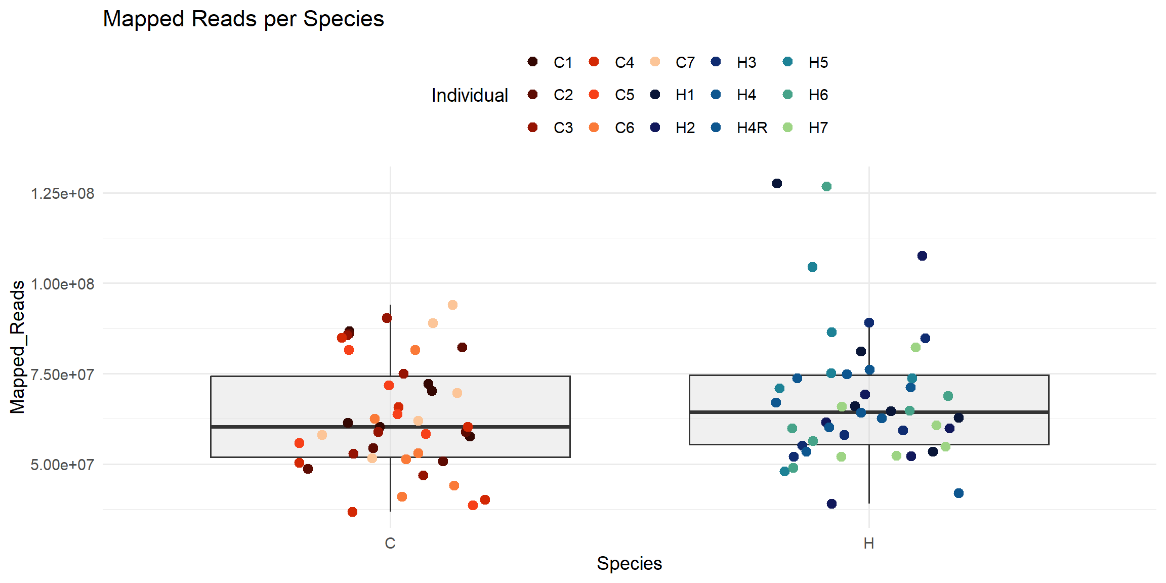
ggplot(total_reads_df, aes(x = Species, y = Mapped_Reads)) +
  geom_boxplot(fill = "#CCCCCC", alpha = 0.3, outlier.shape = NA) +
  geom_jitter(aes(color = Individual), width = 0.2, size = 3) +
  scale_color_manual(values = ann_colors$individual_cor) +
  theme_minimal(base_size = 14) +
  theme(legend.position = "top") +
  labs(
    title = "Mapped Reads per Species",
    x = "Species",
    y = "Mapped_Reads",
    color = "Individual"
  )

Past versions of RNASeq_perSpecies_graph-2.png

Version	Author	Date
0c9c163	John D. Hurley	2026-04-02

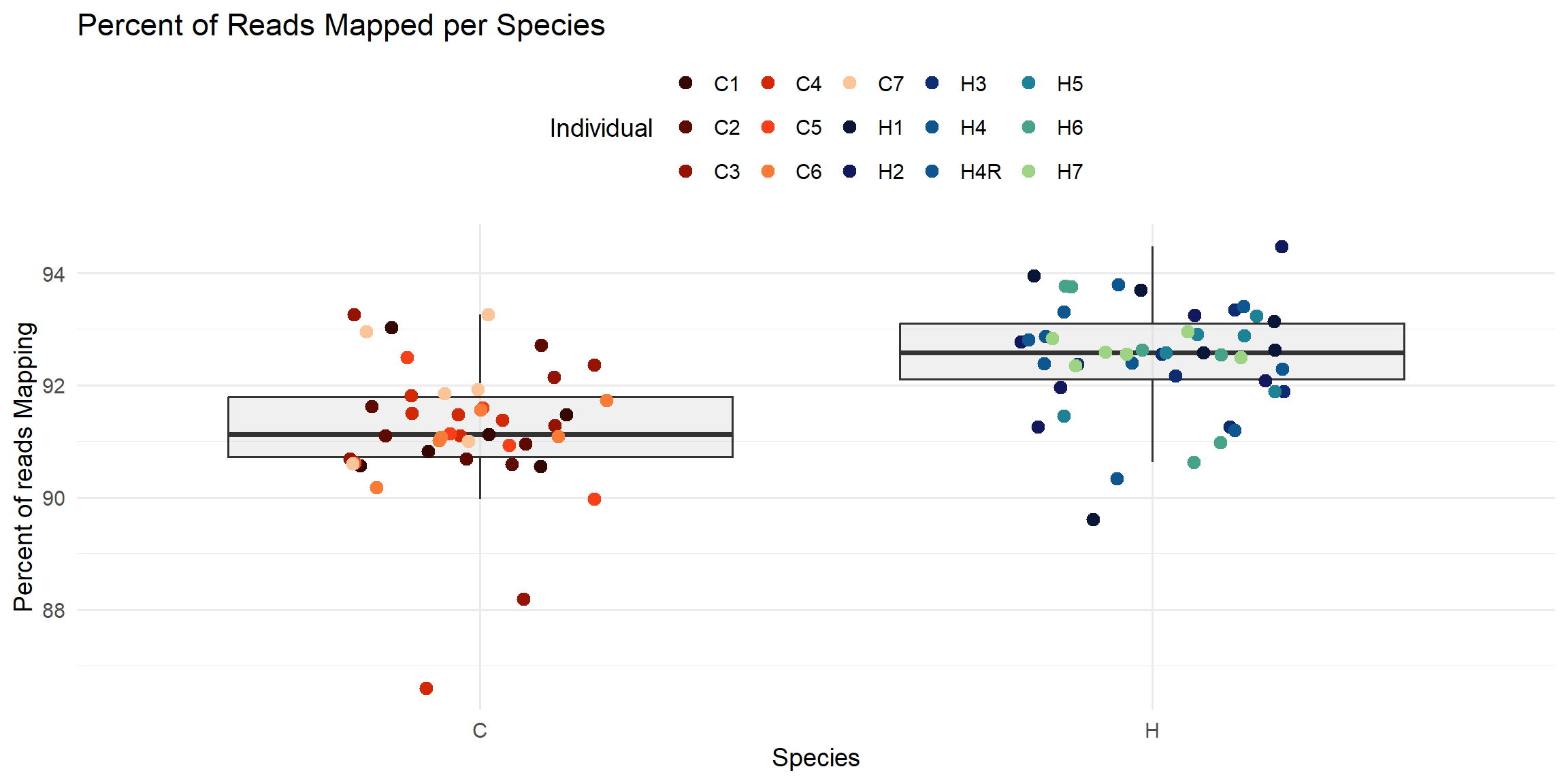
ggplot(total_reads_df, aes(x = Species, y = Percent_Mapped)) +
  geom_boxplot(fill = "#CCCCCC", alpha = 0.3, outlier.shape = NA) +
  geom_jitter(aes(color = Individual), width = 0.2, size = 3) +
  scale_color_manual(values = ann_colors$individual_cor) +
  theme_minimal(base_size = 14) +
  theme(legend.position = "top") +
  labs(
    title = "Percent of Reads Mapped per Species",
    x = "Species",
    y = "Percent of reads Mapping",
    color = "Individual"
  )

Past versions of RNASeq_perSpecies_graph-3.png

Version	Author	Date
0c9c163	John D. Hurley	2026-04-02

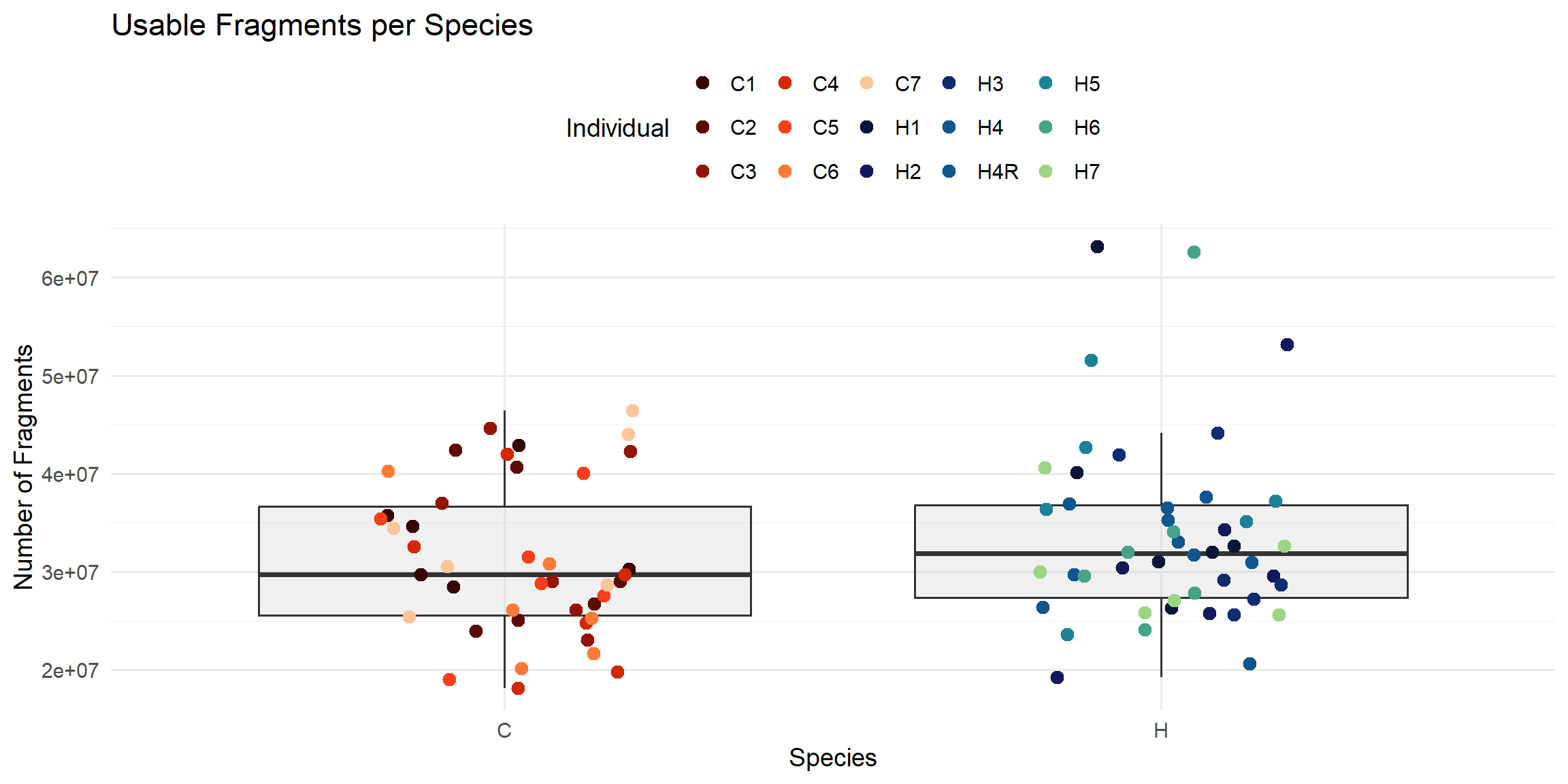
ggplot(total_reads_df, aes(x = Species, y = Usable_Fragments)) +
  geom_boxplot(fill = "#CCCCCC", alpha = 0.3, outlier.shape = NA) +
  geom_jitter(aes(color = Individual), width = 0.2, size = 3) +
  scale_color_manual(values = ann_colors$individual_cor) +
  theme_minimal(base_size = 14) +
  theme(legend.position = "top") +
  labs(
    title = "Usable Fragments per Species",
    x = "Species",
    y = "Number of Fragments",
    color = "Individual"
  )

Past versions of RNASeq_perSpecies_graph-4.png

Version	Author	Date
0c9c163	John D. Hurley	2026-04-02

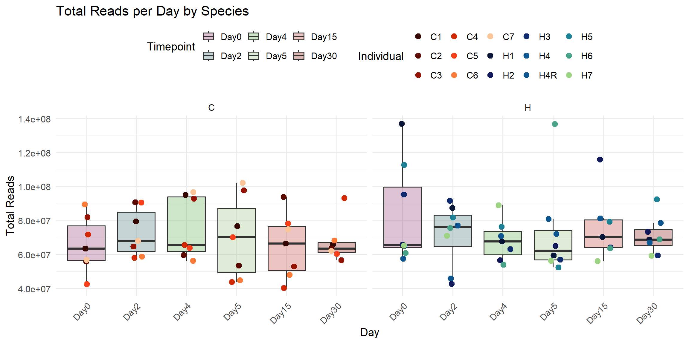
ggplot(total_reads_df, aes(x = Timepoint, y = Total_Reads)) +
  geom_boxplot(aes(fill = Timepoint), alpha = 0.3, outlier.shape = NA) +
  geom_jitter(aes(color = Individual), width = 0.15, size = 3) +
  scale_fill_manual(values = ann_colors$timepoint_cor) +
  scale_color_manual(values = ann_colors$individual_cor) +
  facet_wrap(~Species, scales = "free_x") +
  theme_minimal(base_size = 14) +
  theme(axis.text.x = element_text(angle = 45, hjust = 1),
        legend.position = "top") +
  labs(
    title = "Total Reads per Day by Species",
    x = "Day",
    y = "Total Reads",
    fill = "Timepoint",
    color = "Individual"
  )

Past versions of RNASeq_perDaybySpecies_graph-1.png

Version	Author	Date
0c9c163	John D. Hurley	2026-04-02

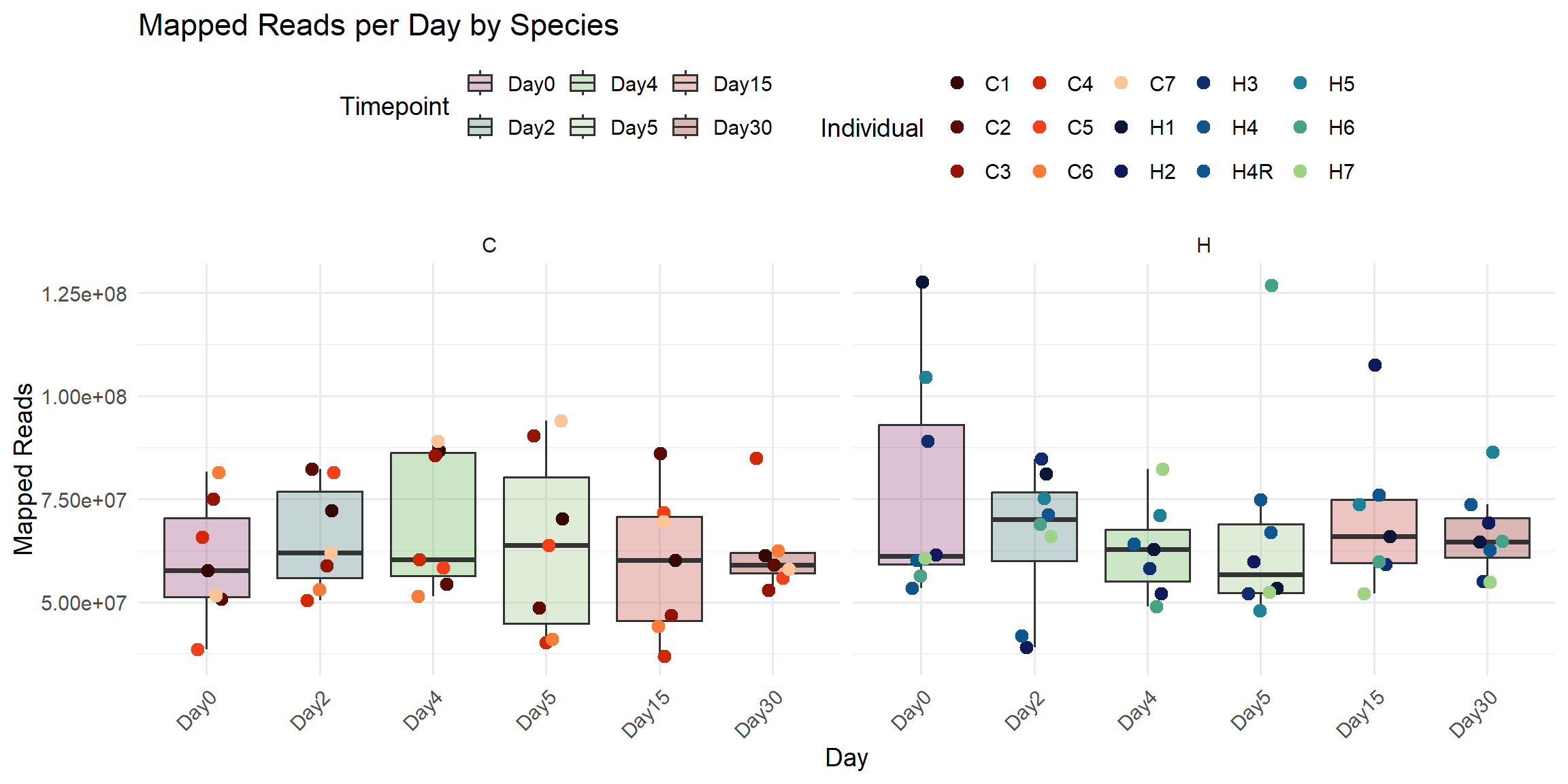
ggplot(total_reads_df, aes(x = Timepoint, y = Mapped_Reads)) +
  geom_boxplot(aes(fill = Timepoint), alpha = 0.3, outlier.shape = NA) +
  geom_jitter(aes(color = Individual), width = 0.15, size = 3) +
  scale_fill_manual(values = ann_colors$timepoint_cor) +
  scale_color_manual(values = ann_colors$individual_cor) +
  facet_wrap(~Species, scales = "free_x") +
  theme_minimal(base_size = 14) +
  theme(axis.text.x = element_text(angle = 45, hjust = 1),
        legend.position = "top") +
  labs(
    title = "Mapped Reads per Day by Species",
    x = "Day",
    y = "Mapped Reads",
    fill = "Timepoint",
    color = "Individual"
  )

Past versions of RNASeq_perDaybySpecies_graph-2.png

Version	Author	Date
0c9c163	John D. Hurley	2026-04-02

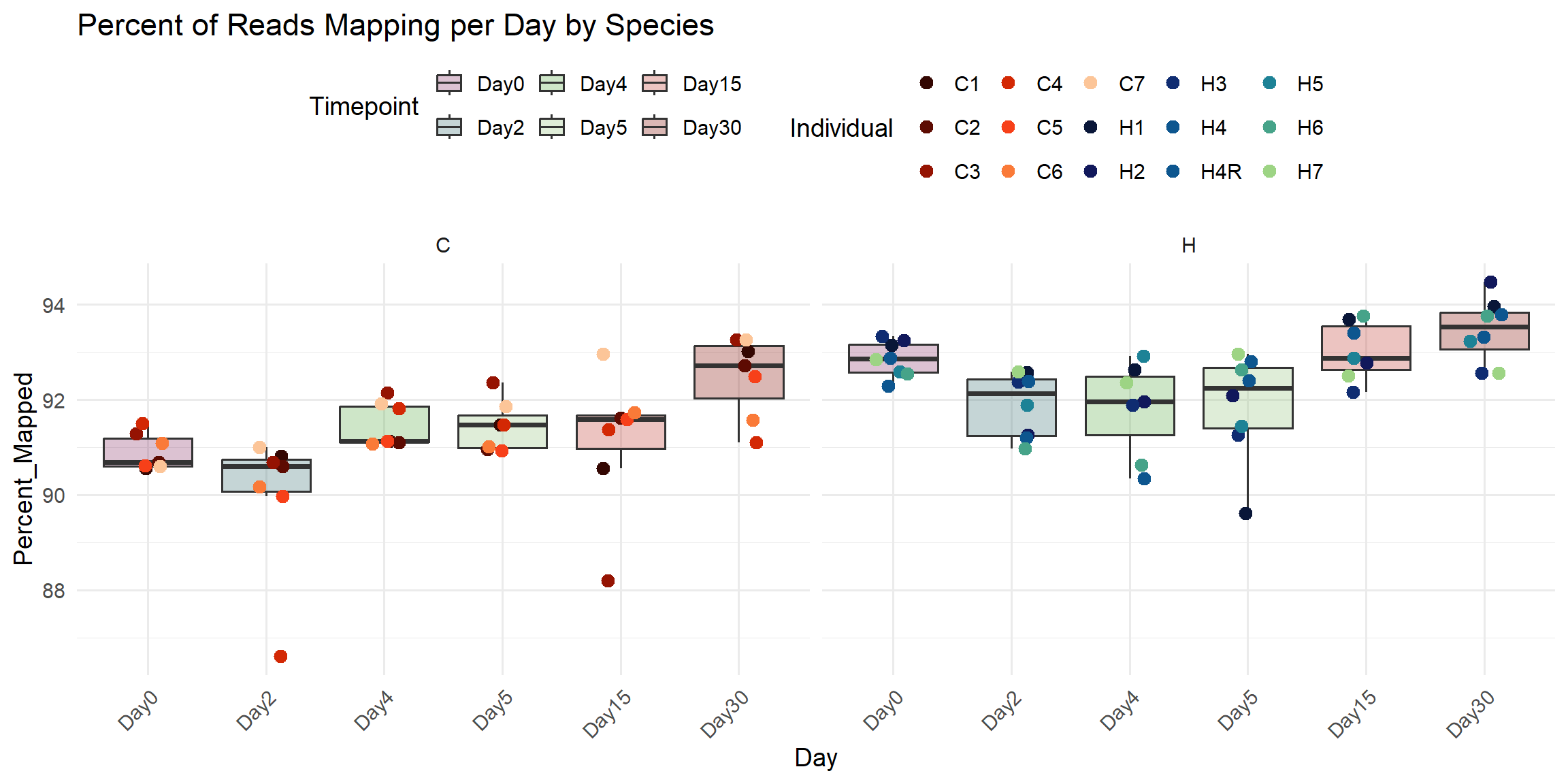
ggplot(total_reads_df, aes(x = Timepoint, y = Percent_Mapped)) +
  geom_boxplot(aes(fill = Timepoint), alpha = 0.3, outlier.shape = NA) +
  geom_jitter(aes(color = Individual), width = 0.15, size = 3) +
  scale_fill_manual(values = ann_colors$timepoint_cor) +
  scale_color_manual(values = ann_colors$individual_cor) +
  facet_wrap(~Species, scales = "free_x") +
  theme_minimal(base_size = 14) +
  theme(axis.text.x = element_text(angle = 45, hjust = 1),
        legend.position = "top") +
  labs(
    title = "Percent of Reads Mapping per Day by Species",
    x = "Day",
    y = "Percent_Mapped",
    fill = "Timepoint",
    color = "Individual"
  )

Past versions of RNASeq_perDaybySpecies_graph-3.png

Version	Author	Date
0c9c163	John D. Hurley	2026-04-02

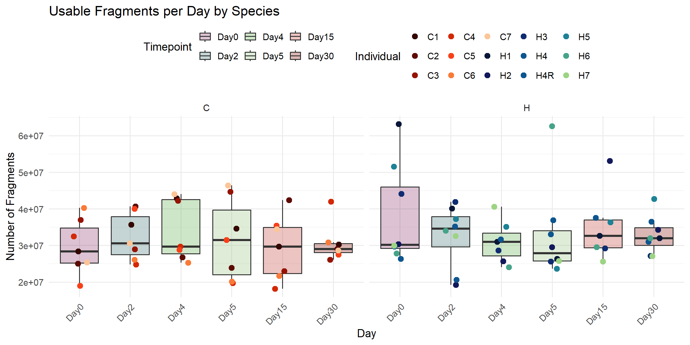
ggplot(total_reads_df, aes(x = Timepoint, y = Usable_Fragments)) +
  geom_boxplot(aes(fill = Timepoint), alpha = 0.3, outlier.shape = NA) +
  geom_jitter(aes(color = Individual), width = 0.15, size = 3) +
  scale_fill_manual(values = ann_colors$timepoint_cor) +
  scale_color_manual(values = ann_colors$individual_cor) +
  facet_wrap(~Species, scales = "free_x") +
  theme_minimal(base_size = 14) +
  theme(axis.text.x = element_text(angle = 45, hjust = 1),
        legend.position = "top") +
  labs(
    title = "Usable Fragments per Day by Species",
    x = "Day",
    y = "Number of Fragments",
    fill = "Timepoint",
    color = "Individual"
  )

Past versions of RNASeq_perDaybySpecies_graph-4.png

Version	Author	Date
0c9c163	John D. Hurley	2026-04-02

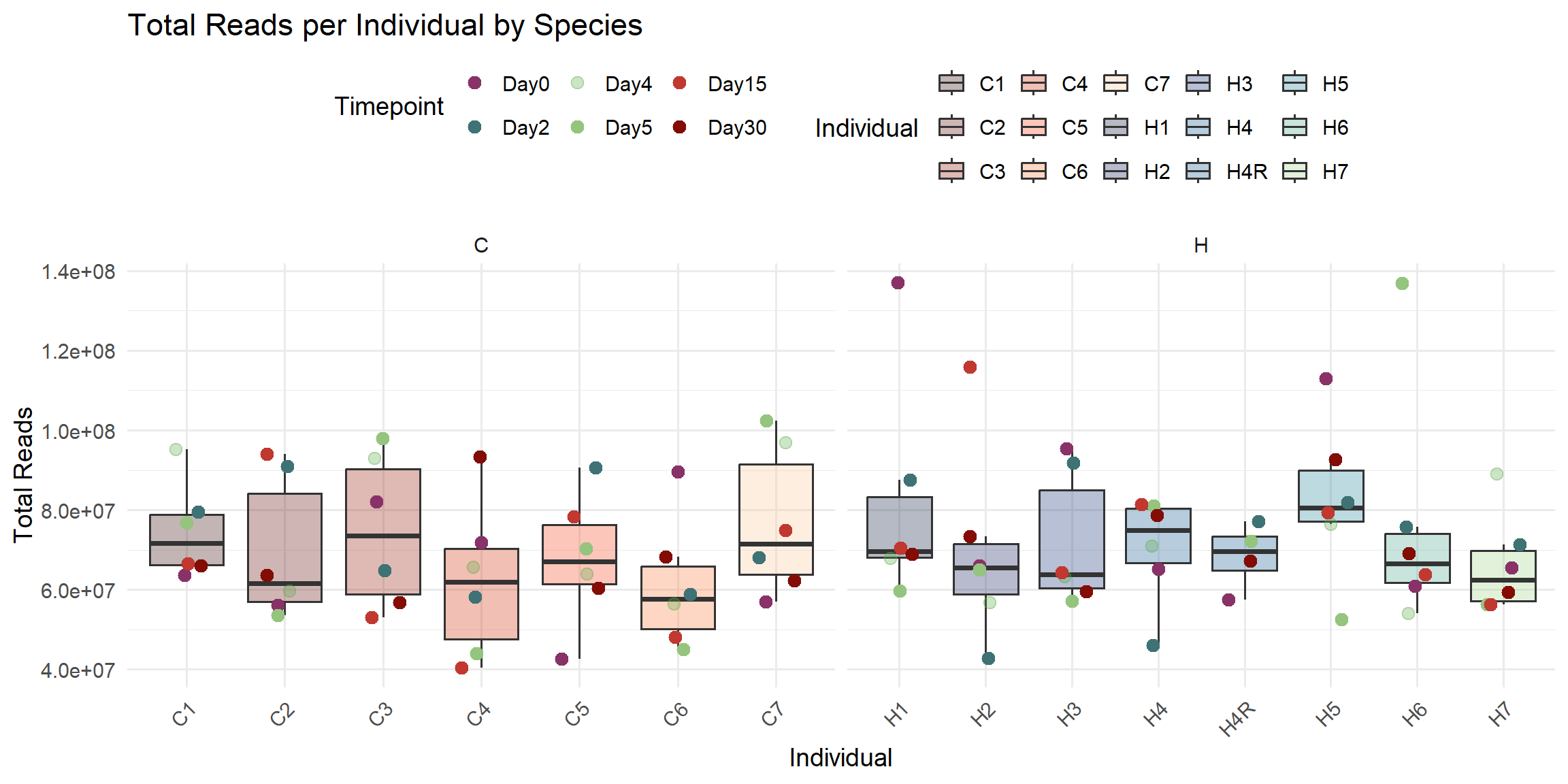
ggplot(total_reads_df, aes(x = Individual, y = Total_Reads)) +
  geom_boxplot(aes(fill = Individual), alpha = 0.3, outlier.shape = NA) +
  geom_jitter(aes(color = Timepoint), width = 0.2, size = 3) +
  scale_fill_manual(values = ann_colors$individual_cor) +
  scale_color_manual(values = ann_colors$timepoint_cor) +
  facet_wrap(~Species, scales = "free_x") +
  theme_minimal(base_size = 14) +
  theme(axis.text.x = element_text(angle = 45, hjust = 1),
        legend.position = "top") +
  labs(
    title = "Total Reads per Individual by Species",
    x = "Individual",
    y = "Total Reads",
    fill = "Individual",
    color = "Timepoint"
  )

Past versions of RNASeq_perIndividualbySpecies_graph-1.png

Version	Author	Date
0c9c163	John D. Hurley	2026-04-02

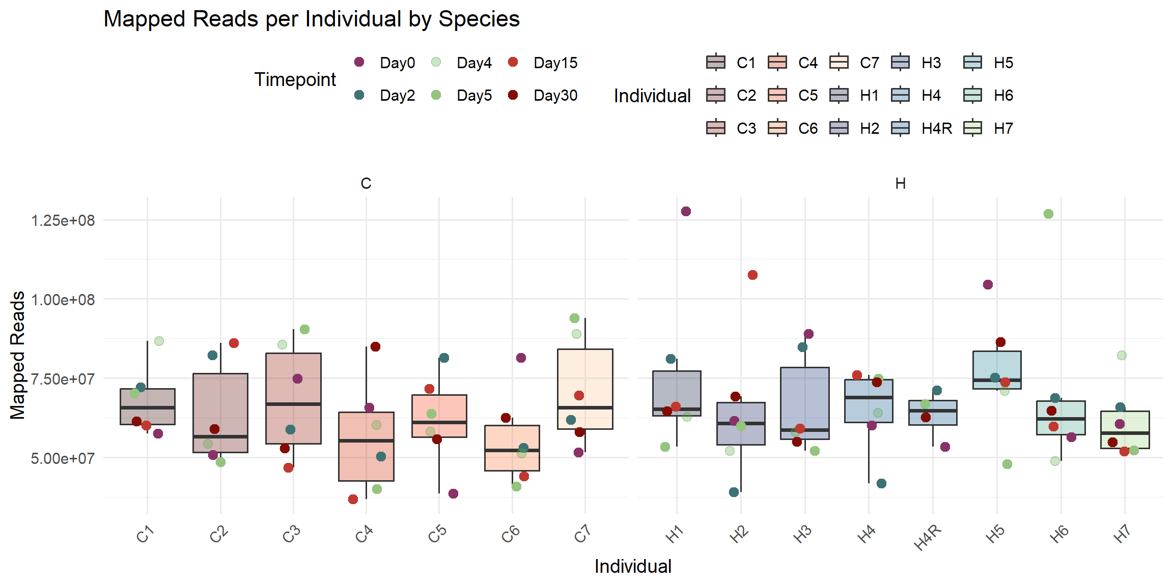
ggplot(total_reads_df, aes(x = Individual, y = Mapped_Reads)) +
  geom_boxplot(aes(fill = Individual), alpha = 0.3, outlier.shape = NA) +
  geom_jitter(aes(color = Timepoint), width = 0.2, size = 3) +
  scale_fill_manual(values = ann_colors$individual_cor) +
  scale_color_manual(values = ann_colors$timepoint_cor) +
  facet_wrap(~Species, scales = "free_x") +
  theme_minimal(base_size = 14) +
  theme(axis.text.x = element_text(angle = 45, hjust = 1),
        legend.position = "top") +
  labs(
    title = "Mapped Reads per Individual by Species",
    x = "Individual",
    y = "Mapped Reads",
    fill = "Individual",
    color = "Timepoint"
  )

Past versions of RNASeq_perIndividualbySpecies_graph-2.png

Version	Author	Date
0c9c163	John D. Hurley	2026-04-02

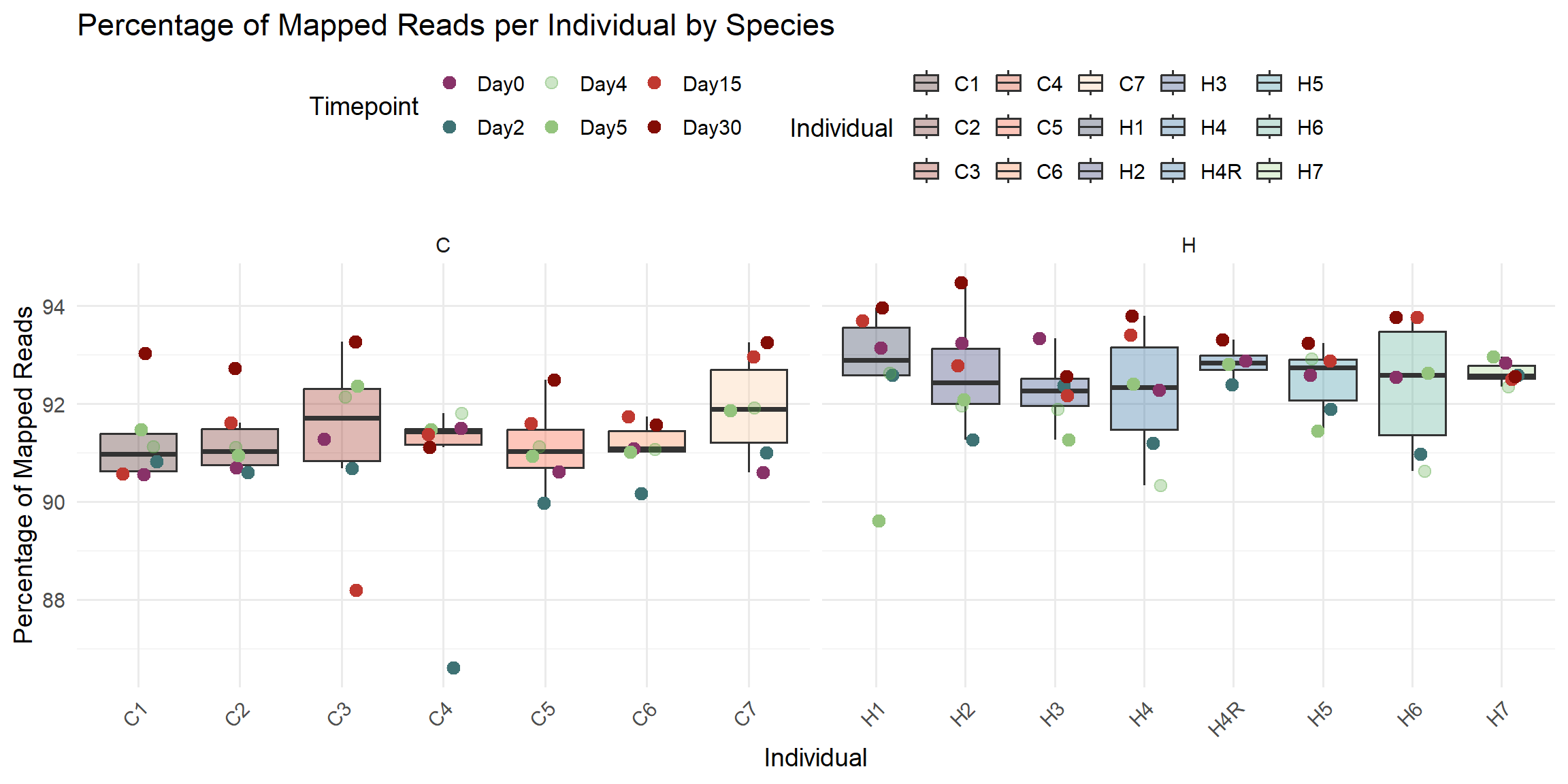
ggplot(total_reads_df, aes(x = Individual, y = Percent_Mapped)) +
  geom_boxplot(aes(fill = Individual), alpha = 0.3, outlier.shape = NA) +
  geom_jitter(aes(color = Timepoint), width = 0.2, size = 3) +
  scale_fill_manual(values = ann_colors$individual_cor) +
  scale_color_manual(values = ann_colors$timepoint_cor) +
  facet_wrap(~Species, scales = "free_x") +
  theme_minimal(base_size = 14) +
  theme(axis.text.x = element_text(angle = 45, hjust = 1),
        legend.position = "top") +
  labs(
    title = "Percentage of Mapped Reads per Individual by Species",
    x = "Individual",
    y = "Percentage of Mapped Reads",
    fill = "Individual",
    color = "Timepoint"
  )

Past versions of RNASeq_perIndividualbySpecies_graph-3.png

Version	Author	Date
0c9c163	John D. Hurley	2026-04-02

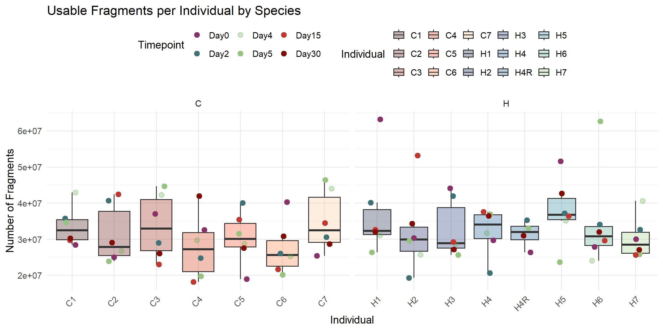
ggplot(total_reads_df, aes(x = Individual, y = Usable_Fragments)) +
  geom_boxplot(aes(fill = Individual), alpha = 0.3, outlier.shape = NA) +
  geom_jitter(aes(color = Timepoint), width = 0.2, size = 3) +
  scale_fill_manual(values = ann_colors$individual_cor) +
  scale_color_manual(values = ann_colors$timepoint_cor) +
  facet_wrap(~Species, scales = "free_x") +
  theme_minimal(base_size = 14) +
  theme(axis.text.x = element_text(angle = 45, hjust = 1),
        legend.position = "top") +
  labs(
    title = "Usable Fragments per Individual by Species",
    x = "Individual",
    y = "Number of Fragments",
    fill = "Individual",
    color = "Timepoint"
  )

Past versions of RNASeq_perIndividualbySpecies_graph-4.png

Version	Author	Date
0c9c163	John D. Hurley	2026-04-02

# -----------------------------
# 1. Prepare long-format data
# -----------------------------
day_levels <- c("Day0","Day2","Day4","Day5","Day15","Day30")
marker_levels <- c("OCT3/4", "Brachy", "ISL-1", "TNNT-2")

RNA_Metadata_NoRep <- RNA_Metadata %>%
  dplyr::filter(!SampleName %in% c(
    "H20682R_Day0",
    "H20682R_Day2",
    "H20682R_Day5",
    "H20682R_Day30"
  ))

df_long_all <- RNA_Metadata_NoRep %>%
  dplyr::select(Individual,Cond, `OCT3/4`, Brachy, `ISL-1`, `TNNT-2`) %>%
  mutate(
    `OCT3/4` = as.numeric(`OCT3/4`),
    Brachy = as.numeric(Brachy),
    `ISL-1` = as.numeric(`ISL-1`),
    `TNNT-2` = as.numeric(`TNNT-2`),
    Group = ifelse(grepl("^H_", Cond), "H", "C")
  ) %>%
  pivot_longer(
    cols = c(`OCT3/4`, Brachy, `ISL-1`, `TNNT-2`),
    names_to = "Marker",
    values_to = "Percent_Positive"
  ) %>%
  mutate(
    Day = gsub(".*_(Day\\d+)$", "\\1", Cond),
    Day = factor(Day, levels = day_levels, ordered = TRUE),
    Marker = factor(Marker, levels = marker_levels, ordered = TRUE)
  )

# -----------------------------
# 2. Compute summary with SEM
# -----------------------------
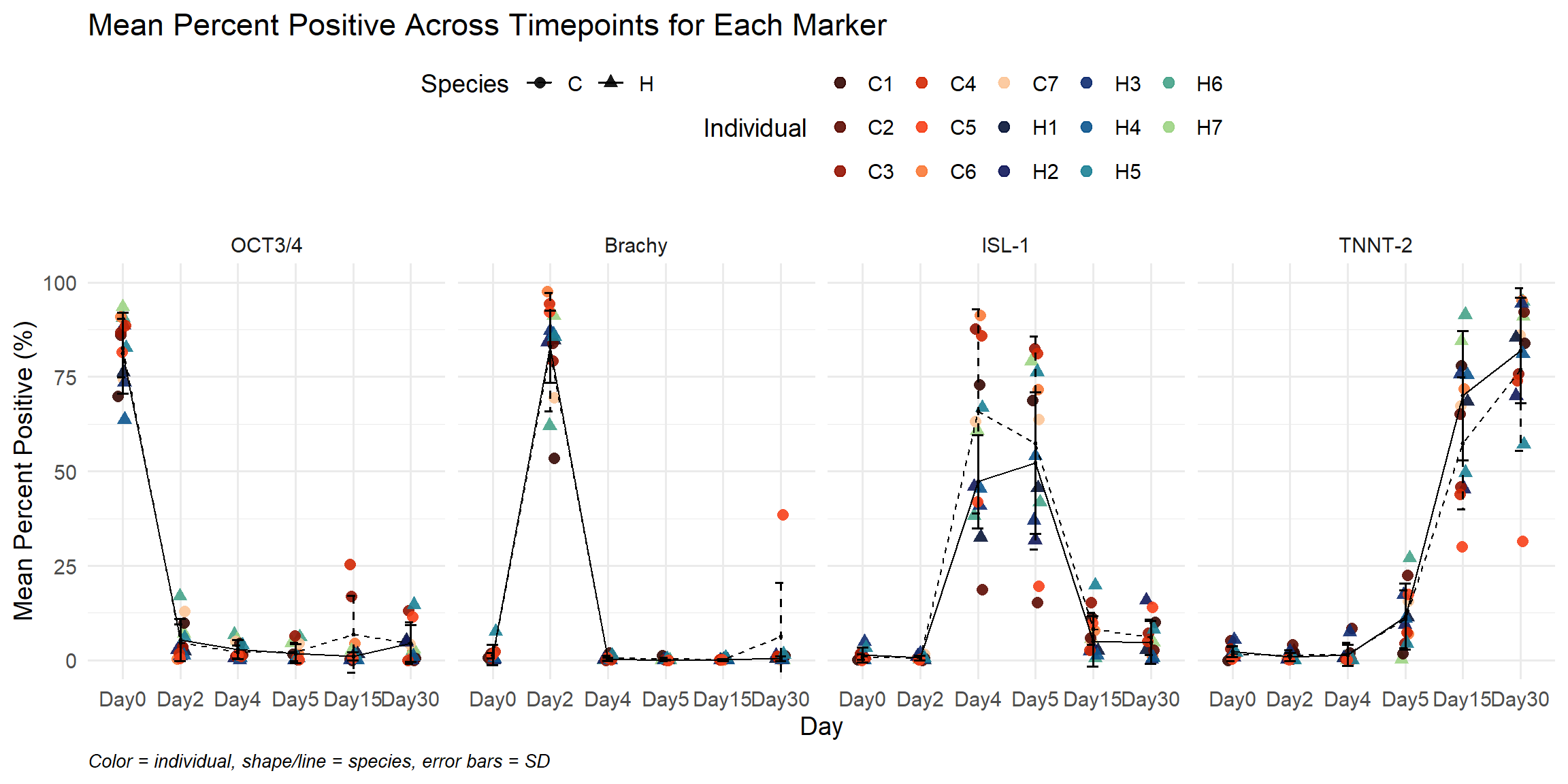
summary_df <- df_long_all %>%
  group_by(Marker, Day, Group) %>%
  summarise(
    Mean = mean(Percent_Positive, na.rm = TRUE),
    SD = sd(Percent_Positive, na.rm = TRUE),
    N = sum(!is.na(Percent_Positive)),
    SEM = SD / sqrt(N),
    .groups = "drop"
  )

# -----------------------------
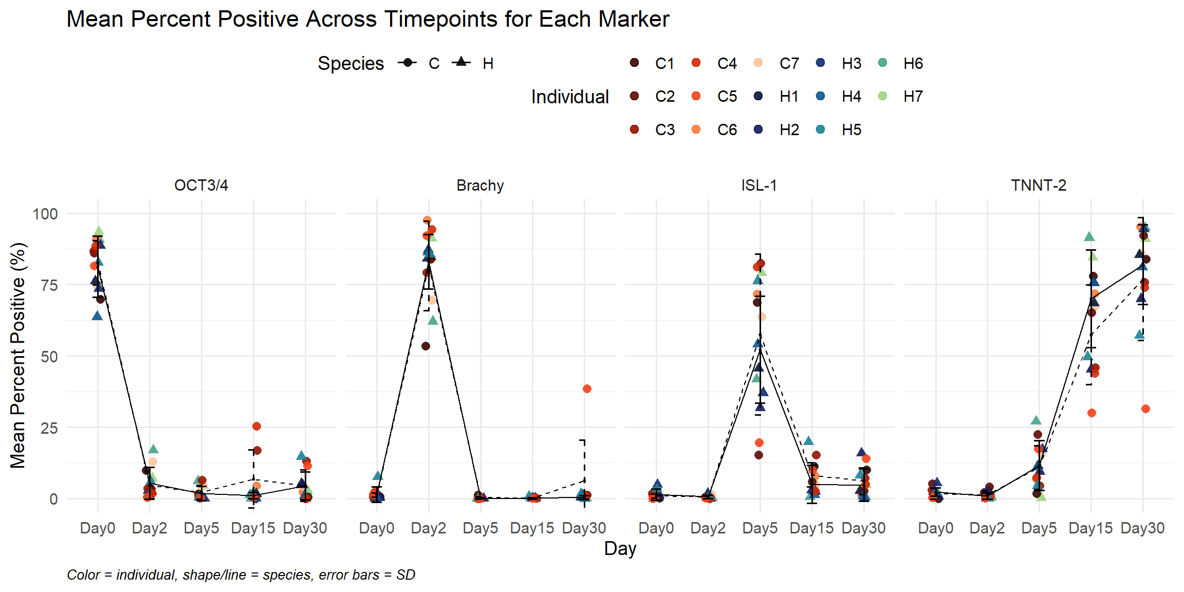
# 3. Plot lines over time with SEM error bars
# -----------------------------
library(dplyr)
library(scales)

ggplot(summary_df,
       aes(x = Day, y = Mean,
           linetype = Group,
           group = Group)) +

  # Individual points
  geom_point(
    data = df_long_all,
    aes(
      x = Day,
      y = Percent_Positive,
      color = Individual,
      shape = Group
    ),
    size = 2.5,
    alpha = 0.9,
    position = position_jitter(width = 0.08, height = 0)
  ) +

  # Mean line (black, texture = species)
  geom_line(
    linewidth = 0.5,
    color = "black"
  ) +

  # Mean point (black)
  geom_point(
    size = 0.5,
    color = "black"
  ) +

  # Error bars (black)
  geom_errorbar(
    aes(ymin = Mean - SD, ymax = Mean + SD),
    width = 0.2,
    color = "black"
  ) +

  facet_wrap(~ Marker, nrow = 1) +

  # species as line texture
  scale_linetype_manual(
    values = c(
      "H" = "solid",
      "C" = "dashed"
    ),
    name = "Species"
  ) +

  # species as shape
  scale_shape_manual(
    values = c(
      "H" = 17,  # triangle
      "C" = 16   # circle
    ),
    name = "Species"
  ) +

  # individual colors from your manual palette
  scale_color_manual(
    values = ann_colors$individual_cor,
    name = "Individual"
  ) +

  # Use coord_cartesian instead of scale_y_continuous to avoid dropped points
  coord_cartesian(ylim = c(0, 100)) +

  labs(
    title = "Mean Percent Positive Across Timepoints for Each Marker",
    x = "Day",
    y = "Mean Percent Positive (%)",
    caption = "Color = individual, shape/line = species, error bars = SD"
  ) +

  theme_minimal(base_size = 14) +
  theme(
    legend.position = "top",
    axis.text.x = element_text(angle = 0, hjust = 0.5),
    plot.caption = element_text(hjust = 0, face = "italic", size = 10)
  )

Past versions of RNASeq_Purities_graph-1.png

Version	Author	Date
0958201	John D. Hurley	2026-03-23
fcf8fc0	John D. Hurley	2026-02-18

# -----------------------------
# 1. Prepare long-format data
# -----------------------------
day_levels <- c("Day0","Day2","Day4","Day5","Day15","Day30")
marker_levels <- c("OCT3/4", "Brachy", "ISL-1", "TNNT-2")

RNA_Metadata_NoD4_NoRep <- RNA_Metadata %>%
  dplyr::filter(Timepoint != "Day4") %>%
  dplyr::filter(!SampleName %in% c(
    "H20682R_Day0",
    "H20682R_Day2",
    "H20682R_Day5",
    "H20682R_Day30"
  ))

df_long_No4 <- RNA_Metadata_NoD4_NoRep %>%
  dplyr::select(Individual,Cond, `OCT3/4`, Brachy, `ISL-1`, `TNNT-2`) %>%
  mutate(
    `OCT3/4` = as.numeric(`OCT3/4`),
    Brachy = as.numeric(Brachy),
    `ISL-1` = as.numeric(`ISL-1`),
    `TNNT-2` = as.numeric(`TNNT-2`),
    Group = ifelse(grepl("^H_", Cond), "H", "C")
  ) %>%
  pivot_longer(
    cols = c(`OCT3/4`, Brachy, `ISL-1`, `TNNT-2`),
    names_to = "Marker",
    values_to = "Percent_Positive"
  ) %>%
  mutate(
    Day = gsub(".*_(Day\\d+)$", "\\1", Cond),
    Day = factor(Day, levels = day_levels, ordered = TRUE),
    Marker = factor(Marker, levels = marker_levels, ordered = TRUE)
  )

# -----------------------------
# 2. Compute summary with SEM
# -----------------------------
summary_df_No4 <- df_long_No4 %>%
  group_by(Marker, Day, Group) %>%
  summarise(
    Mean = mean(Percent_Positive, na.rm = TRUE),
    SD = sd(Percent_Positive, na.rm = TRUE),
    N = sum(!is.na(Percent_Positive)),
    SEM = SD / sqrt(N),
    .groups = "drop"
  )

# -----------------------------
# 3. Plot lines over time with SEM error bars
# -----------------------------
library(dplyr)
library(scales)

ggplot(summary_df_No4,
       aes(x = Day, y = Mean,
           linetype = Group,
           group = Group)) +

  # Individual points
  geom_point(
    data = df_long_No4,
    aes(
      x = Day,
      y = Percent_Positive,
      color = Individual,
      shape = Group
    ),
    size = 2.5,
    alpha = 0.9,
    position = position_jitter(width = 0.08, height = 0)
  ) +

  # Mean line (black, texture = species)
  geom_line(
    linewidth = 0.5,
    color = "black"
  ) +

  # Mean point (black)
  geom_point(
    size = 0.5,
    color = "black"
  ) +

  # Error bars (black)
  geom_errorbar(
    aes(ymin = Mean - SD, ymax = Mean + SD),
    width = 0.2,
    color = "black"
  ) +

  facet_wrap(~ Marker, nrow = 1) +

  # species as line texture
  scale_linetype_manual(
    values = c(
      "H" = "solid",
      "C" = "dashed"
    ),
    name = "Species"
  ) +

  # species as shape
  scale_shape_manual(
    values = c(
      "H" = 17,  # triangle
      "C" = 16   # circle
    ),
    name = "Species"
  ) +

  # individual colors from your manual palette
  scale_color_manual(
    values = ann_colors$individual_cor,
    name = "Individual"
  ) +

  # Use coord_cartesian instead of scale_y_continuous to avoid dropped points
  coord_cartesian(ylim = c(0, 100)) +

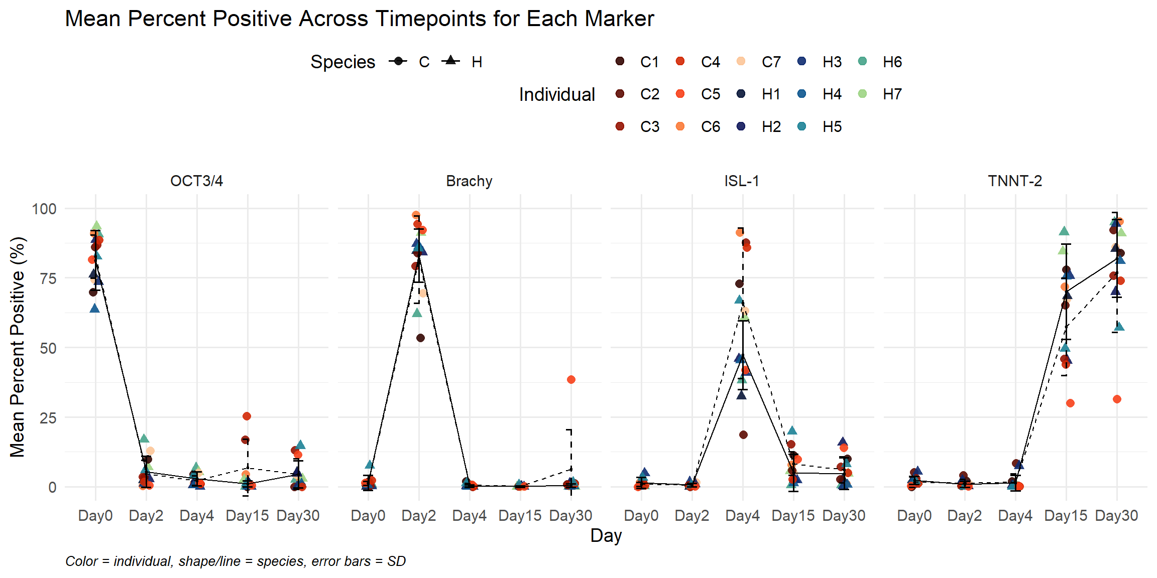
  labs(
    title = "Mean Percent Positive Across Timepoints for Each Marker",
    x = "Day",
    y = "Mean Percent Positive (%)",
    caption = "Color = individual, shape/line = species, error bars = SD"
  ) +

  theme_minimal(base_size = 14) +
  theme(
    legend.position = "top",
    axis.text.x = element_text(angle = 0, hjust = 0.5),
    plot.caption = element_text(hjust = 0, face = "italic", size = 10)
  )

Past versions of RNASeq_Purities_graph_No4_graph-1.png

Version	Author	Date
0c9c163	John D. Hurley	2026-04-02

# -----------------------------
# 1. Prepare long-format data
# -----------------------------
day_levels <- c("Day0","Day2","Day4","Day5","Day15","Day30")
marker_levels <- c("OCT3/4", "Brachy", "ISL-1", "TNNT-2")

RNA_Metadata_NoD5_NoRep <- RNA_Metadata %>%
  dplyr::filter(Timepoint != "Day5") %>%
  dplyr::filter(!SampleName %in% c(
    "H20682R_Day0",
    "H20682R_Day2",
    "H20682R_Day5",
    "H20682R_Day30"
  ))

df_long_No5 <- RNA_Metadata_NoD5_NoRep %>%
  dplyr::select(Individual,Cond, `OCT3/4`, Brachy, `ISL-1`, `TNNT-2`) %>%
  mutate(
    `OCT3/4` = as.numeric(`OCT3/4`),
    Brachy = as.numeric(Brachy),
    `ISL-1` = as.numeric(`ISL-1`),
    `TNNT-2` = as.numeric(`TNNT-2`),
    Group = ifelse(grepl("^H_", Cond), "H", "C")
  ) %>%
  pivot_longer(
    cols = c(`OCT3/4`, Brachy, `ISL-1`, `TNNT-2`),
    names_to = "Marker",
    values_to = "Percent_Positive"
  ) %>%
  mutate(
    Day = gsub(".*_(Day\\d+)$", "\\1", Cond),
    Day = factor(Day, levels = day_levels, ordered = TRUE),
    Marker = factor(Marker, levels = marker_levels, ordered = TRUE)
  )

# -----------------------------
# 2. Compute summary with SEM
# -----------------------------
summary_df_No5 <- df_long_No5 %>%
  group_by(Marker, Day, Group) %>%
  summarise(
    Mean = mean(Percent_Positive, na.rm = TRUE),
    SD = sd(Percent_Positive, na.rm = TRUE),
    N = sum(!is.na(Percent_Positive)),
    SEM = SD / sqrt(N),
    .groups = "drop"
  )

# -----------------------------
# 3. Plot lines over time with SEM error bars
# -----------------------------
library(dplyr)
library(scales)

ggplot(summary_df_No5,
       aes(x = Day, y = Mean,
           linetype = Group,
           group = Group)) +

  # Individual points
  geom_point(
    data = df_long_No5,
    aes(
      x = Day,
      y = Percent_Positive,
      color = Individual,
      shape = Group
    ),
    size = 2.5,
    alpha = 0.9,
    position = position_jitter(width = 0.08, height = 0)
  ) +

  # Mean line (black, texture = species)
  geom_line(
    linewidth = 0.5,
    color = "black"
  ) +

  # Mean point (black)
  geom_point(
    size = 0.5,
    color = "black"
  ) +

  # Error bars (black)
  geom_errorbar(
    aes(ymin = Mean - SD, ymax = Mean + SD),
    width = 0.2,
    color = "black"
  ) +

  facet_wrap(~ Marker, nrow = 1) +

  # species as line texture
  scale_linetype_manual(
    values = c(
      "H" = "solid",
      "C" = "dashed"
    ),
    name = "Species"
  ) +

  # species as shape
  scale_shape_manual(
    values = c(
      "H" = 17,  # triangle
      "C" = 16   # circle
    ),
    name = "Species"
  ) +

  # individual colors from your manual palette
  scale_color_manual(
    values = ann_colors$individual_cor,
    name = "Individual"
  ) +

  # Use coord_cartesian instead of scale_y_continuous to avoid dropped points
  coord_cartesian(ylim = c(0, 100)) +

  labs(
    title = "Mean Percent Positive Across Timepoints for Each Marker",
    x = "Day",
    y = "Mean Percent Positive (%)",
    caption = "Color = individual, shape/line = species, error bars = SD"
  ) +

  theme_minimal(base_size = 14) +
  theme(
    legend.position = "top",
    axis.text.x = element_text(angle = 0, hjust = 0.5),
    plot.caption = element_text(hjust = 0, face = "italic", size = 10)
  )

Past versions of RNASeq_Purities_graph_No5_graph-1.png

Version	Author	Date
0c9c163	John D. Hurley	2026-04-02

#####Unfiltered####
RNA_log2cpm <- cpm(RNA_fc, log = TRUE)

hist(RNA_log2cpm,  main = "Histogram of all counts (unfiltered)",
     xlab =expression("Log"[2]*" counts-per-million"), col =4 )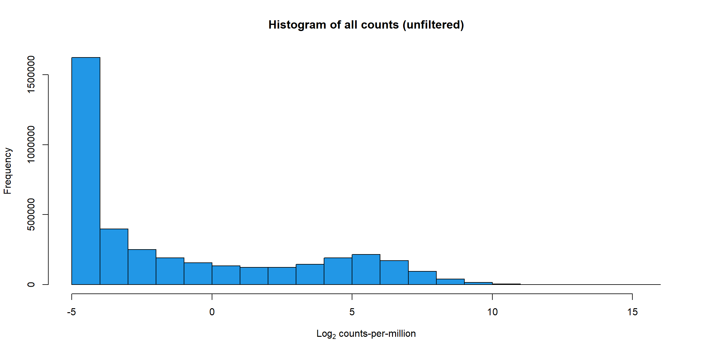

Past versions of RNASeq_FeatureCounts_Box_Unfiltered-1.png

Version	Author	Date
0958201	John D. Hurley	2026-03-23
fcf8fc0	John D. Hurley	2026-02-18
7789dff	John D. Hurley	2026-01-28
d9f15a6	John D. Hurley	2026-01-28

boxplot(RNA_log2cpm, main = "Boxplots of log cpm per sample
          (unfiltered)", xaxt = "n", xlab= "")
axis(1,
     at = 1:length(col_names),  # positions (one per sample)
     labels = col_names,        # your labels vector
     las = 2,               # rotate text vertically (like srt=90)
     cex.axis = 0.6)        # shrink label size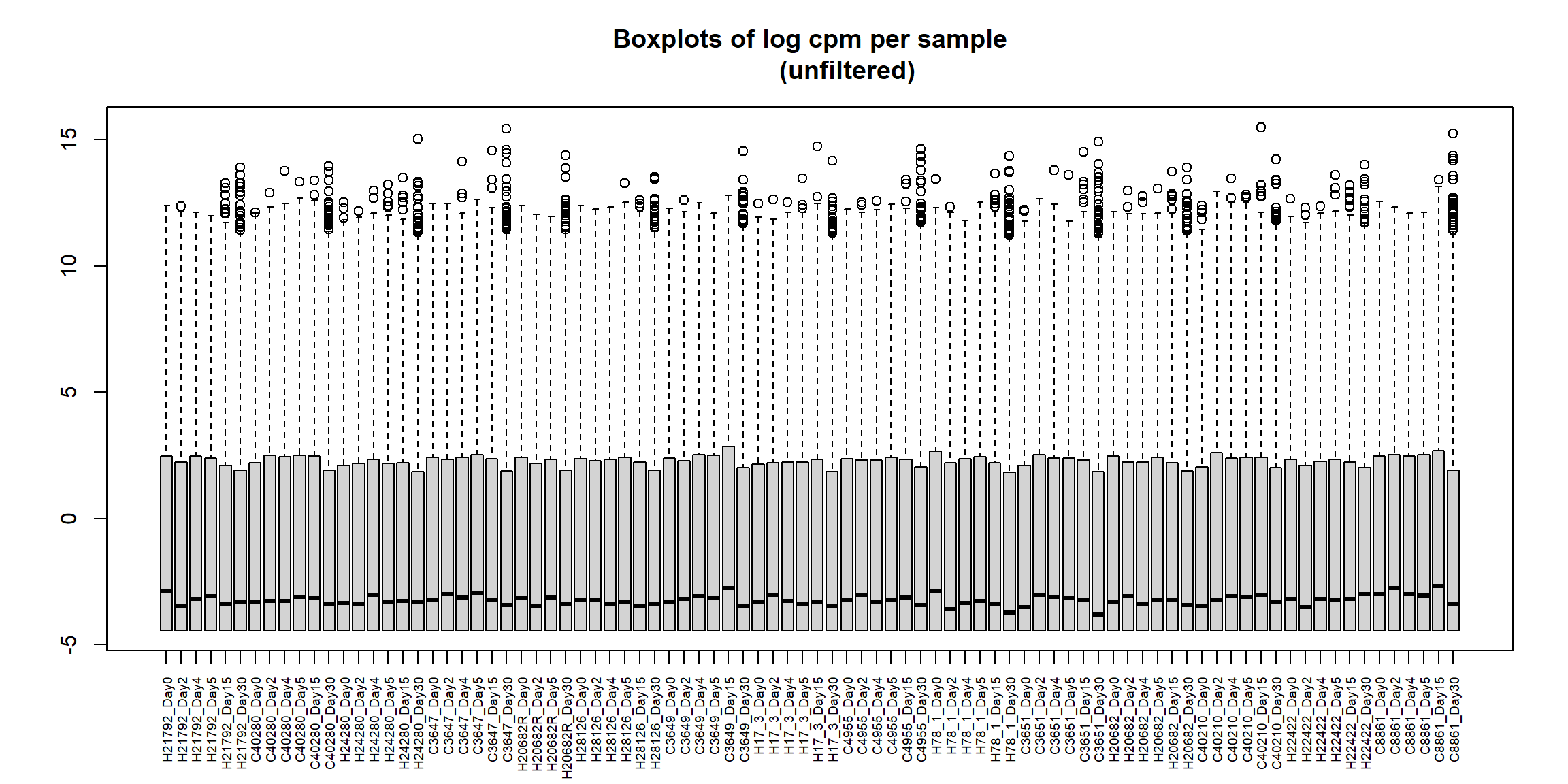

Past versions of RNASeq_FeatureCounts_Box_Unfiltered-2.png

Version	Author	Date
0958201	John D. Hurley	2026-03-23
fcf8fc0	John D. Hurley	2026-02-18
7789dff	John D. Hurley	2026-01-28
d9f15a6	John D. Hurley	2026-01-28

# saveRDS(RNA_log2cpm,"data/QC/concat/RNA_log2cpm.RDS")

#####RowMu>0####
row_means <- rowMeans(RNA_log2cpm)
Filt_RMG0_RNA_fc <- RNA_fc[row_means >0,]

# saveRDS(Filt_RMG0_RNA_fc,"data/QC/concat/Filt_RMG0_RNA_fc.RDS")

Filt_RMG0_RNA_log2cpm <- cpm(Filt_RMG0_RNA_fc,log=TRUE)

# saveRDS(Filt_RMG0_RNA_log2cpm,"data/QC/concat/Filt_RMG0_RNA_log2cpm.RDS")

hist(Filt_RMG0_RNA_log2cpm, main = "Histogram of filtered counts using rowMeans > 0 method",
     xlab =expression("Log"[2]*" counts-per-million"), col =5 )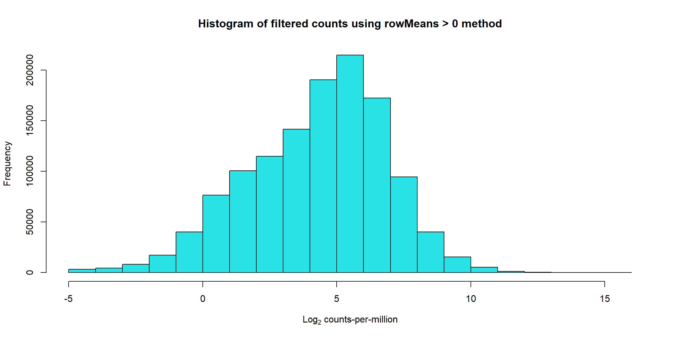

Past versions of RNASeq_FeatureCounts_RMG0-1.png

Version	Author	Date
0958201	John D. Hurley	2026-03-23
7789dff	John D. Hurley	2026-01-28
d9f15a6	John D. Hurley	2026-01-28

boxplot(Filt_RMG0_RNA_log2cpm, main = "Boxplots of log cpm per sample (RowMeans>0)",xaxt = "n", xlab= "")
axis(1,
     at = 1:length(col_names),  # positions (one per sample)
     labels = col_names,        # your labels vector
     las = 2,               # rotate text vertically (like srt=90)
     cex.axis = 0.6)        # shrink label size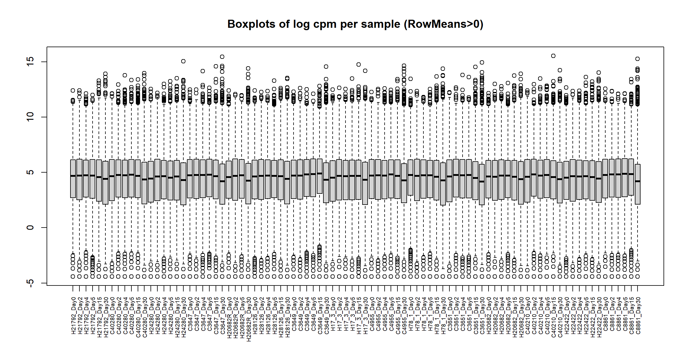

Past versions of RNASeq_FeatureCounts_Box_RMG0-1.png

Version	Author	Date
0958201	John D. Hurley	2026-03-23
7789dff	John D. Hurley	2026-01-28
d9f15a6	John D. Hurley	2026-01-28

library(ggplot2)
library(dplyr)

# Define ordered day factor
day_levels <- c("Day0", "Day2", "Day4", "Day5", "Day15", "Day30")

total_reads_df <- total_reads_df %>%
  mutate(
    # Order Timepoint for bars
    Timepoint = factor(Timepoint, levels = day_levels, ordered = TRUE),
    
    # Individual text color
    Individual_Color = ann_colors$individual_cor[Individual]
  ) %>%
  # Order Sample for x-axis: first by Individual, then by Day
  arrange(Individual, Timepoint) %>%
  mutate(Sample = factor(Sample, levels = Sample))  # preserve order in ggplot

# Plot
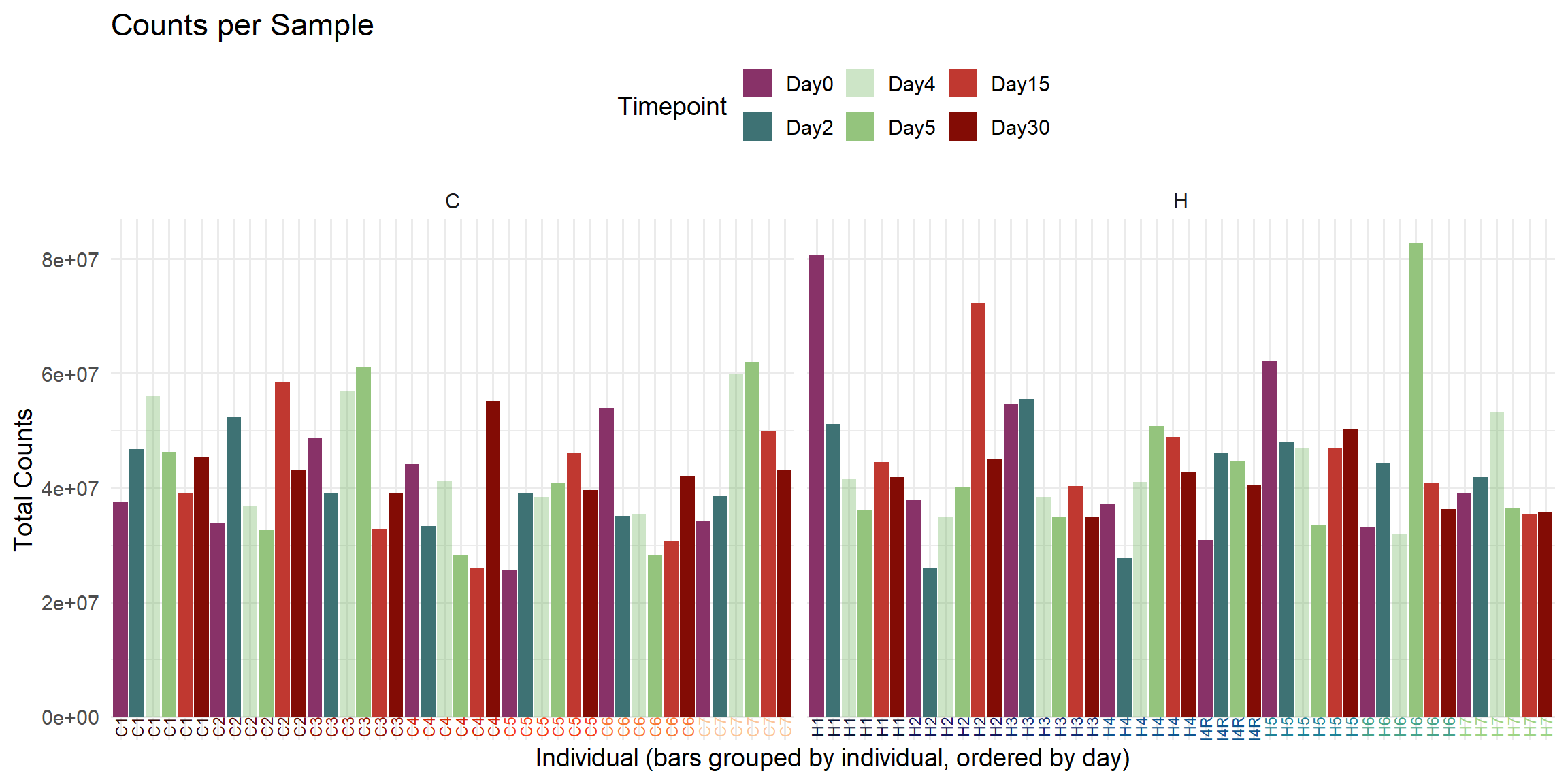
ggplot(total_reads_df, aes(x = Sample, y = Total_Counts, fill = Timepoint)) +
  
  # Bars colored by Timepoint
  geom_col() +

  # Annotate Individual names under bars, colored by individual
  geom_text(
    aes(label = Individual, color = Individual_Color),
    y = 0, angle = 90, hjust = 1, vjust = 0.5, size = 3
  ) +

  # Manual Timepoint colors
  scale_fill_manual(values = ann_colors$timepoint_cor) +

  # Use exact color for individual labels
  scale_color_identity() +

  # Facet by Species if desired
  facet_grid(~Species, scales = "free_x", space = "free_x") +

  # Theme
  theme_minimal(base_size = 14) +
  theme(
    axis.text.x = element_blank(),  # hide default X labels
    axis.ticks.x = element_blank(),
    legend.position = "top"
  ) +

  labs(
    title = "Counts per Sample",
    x = "Individual (bars grouped by individual, ordered by day)",
    y = "Total Counts",
    fill = "Timepoint"
  )

Past versions of RNASeq_Counts_graph-1.png

Version	Author	Date
0c9c163	John D. Hurley	2026-04-02

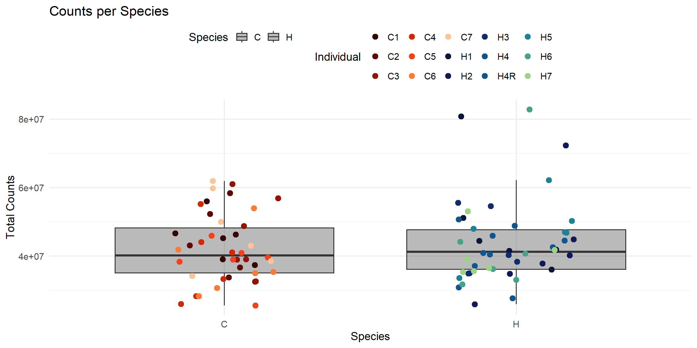
ggplot(total_reads_df, aes(x = Species, y = Total_Counts)) +
  
  # Boxplot for each species
  geom_boxplot(aes(fill = Species), alpha = 0.3, outlier.shape = NA) + 
  
  # Overlay individual points colored by individual
  geom_jitter(aes(color = Individual), width = 0.2, size = 3) +

  # Use individual colors
  scale_color_manual(values = ann_colors$individual_cor) +

  # Optional: species fill colors (light grey / black)
  scale_fill_manual(values = c("H" = "#17171717", "C" = "#17171717")) +

  theme_minimal(base_size = 14) +
  theme(
    legend.position = "top"
  ) +

  labs(
    title = "Counts per Species",
    x = "Species",
    y = "Total Counts",
    color = "Individual",
    fill = "Species"
  )

Past versions of RNASeq_Counts_graph-2.png

Version	Author	Date
0c9c163	John D. Hurley	2026-04-02

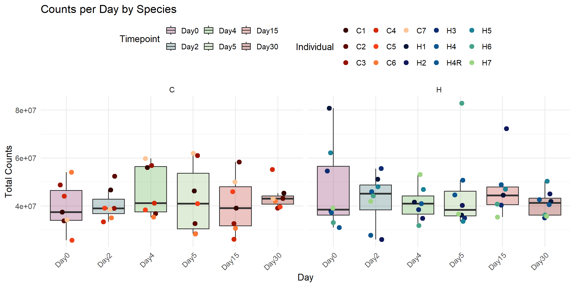
ggplot(total_reads_df, aes(x = Timepoint, y = Total_Counts)) +
  
  # Boxplot per day
  geom_boxplot(aes(fill = Timepoint), alpha = 0.3, outlier.shape = NA) +

  # Overlay individual points colored by individual
  geom_jitter(aes(color = Individual), width = 0.15, size = 3) +

  # Use individual colors
  scale_color_manual(values = ann_colors$individual_cor) +

  # Use timepoint colors for boxplots
  scale_fill_manual(values = ann_colors$timepoint_cor) +

  # Separate x-axis by species
  facet_wrap(~Species, scales = "free_x") +

  theme_minimal(base_size = 14) +
  theme(
    legend.position = "top",
    axis.text.x = element_text(angle = 45, hjust = 1)
  ) +

  labs(
    title = "Counts per Day by Species",
    x = "Day",
    y = "Total Counts",
    color = "Individual",
    fill = "Timepoint"
  )

Past versions of RNASeq_Counts_graph-3.png

Version	Author	Date
0c9c163	John D. Hurley	2026-04-02

# Plot
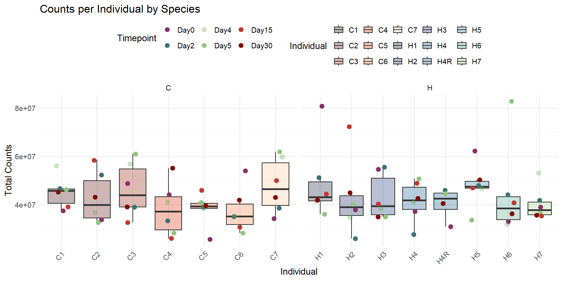
ggplot(total_reads_df, aes(x = Individual, y = Total_Counts)) +
  
  # Boxplots colored by individual
  geom_boxplot(aes(fill = Individual), alpha = 0.3, outlier.shape = NA) +

  # Overlay points colored by Timepoint
  geom_jitter(aes(color = Timepoint), width = 0.2, size = 3) +

  # Use manual colors
  scale_fill_manual(values = ann_colors$individual_cor) +
  scale_color_manual(values = ann_colors$timepoint_cor) +

  # Facet by species
  facet_wrap(~Species, scales = "free_x", nrow = 1) +

  # Theme
  theme_minimal(base_size = 14) +
  theme(
    legend.position = "top",
    axis.text.x = element_text(angle = 45, hjust = 1)
  ) +

  labs(
    title = "Counts per Individual by Species",
    x = "Individual",
    y = "Total Counts",
    fill = "Individual",
    color = "Timepoint"
  )

Past versions of RNASeq_Counts_graph-4.png

Version	Author	Date
0c9c163	John D. Hurley	2026-04-02

library(tidyverse)

total_reads_df <- RNA_fc %>%
  as.data.frame() %>%
  mutate(Gene = rownames(.)) %>%
  dplyr::select(-Gene) %>%
  summarise(across(everything(), \(x) sum(x, na.rm = TRUE))) %>%
  pivot_longer(
    cols = everything(),
    names_to = "Sample",
    values_to = "Total_Reads"
  ) %>%
  left_join(RNA_Metadata, by = c("Sample" = "SampleName"))

library(ggplot2)
library(dplyr)

# Define ordered day factor
day_levels <- c("Day0", "Day2", "Day4", "Day5", "Day15", "Day30")

total_reads_df <- total_reads_df %>%
  mutate(
    # Order Timepoint for bars
    Timepoint = factor(Timepoint, levels = day_levels, ordered = TRUE),
    
    # Individual text color
    Individual_Color = ann_colors$individual_cor[Individual]
  ) %>%
  # Order Sample for x-axis: first by Individual, then by Day
  arrange(Individual, Timepoint) %>%
  mutate(Sample = factor(Sample, levels = Sample))  # preserve order in ggplot

# Plot
ggplot(total_reads_df, aes(x = Sample, y = Total_Reads.x, fill = Timepoint)) +
  
  # Bars colored by Timepoint
  geom_col() +

  # Annotate Individual names under bars, colored by individual
  geom_text(
    aes(label = Individual, color = Individual_Color),
    y = 0, angle = 90, hjust = 1, vjust = 0.5, size = 3
  ) +

  # Manual Timepoint colors
  scale_fill_manual(values = ann_colors$timepoint_cor) +

  # Use exact color for individual labels
  scale_color_identity() +

  # Facet by Species if desired
  facet_grid(~Species, scales = "free_x", space = "free_x") +

  # Theme
  theme_minimal(base_size = 14) +
  theme(
    axis.text.x = element_blank(),  # hide default X labels
    axis.ticks.x = element_blank(),
    legend.position = "top"
  ) +

  labs(
    title = "Total Reads per Sample",
    x = "Individual (bars grouped by individual, ordered by day)",
    y = "Total Reads",
    fill = "Timepoint"
  )

Past versions of RNASeq_TotalReads_graph-1.png

Version	Author	Date
0c9c163	John D. Hurley	2026-04-02

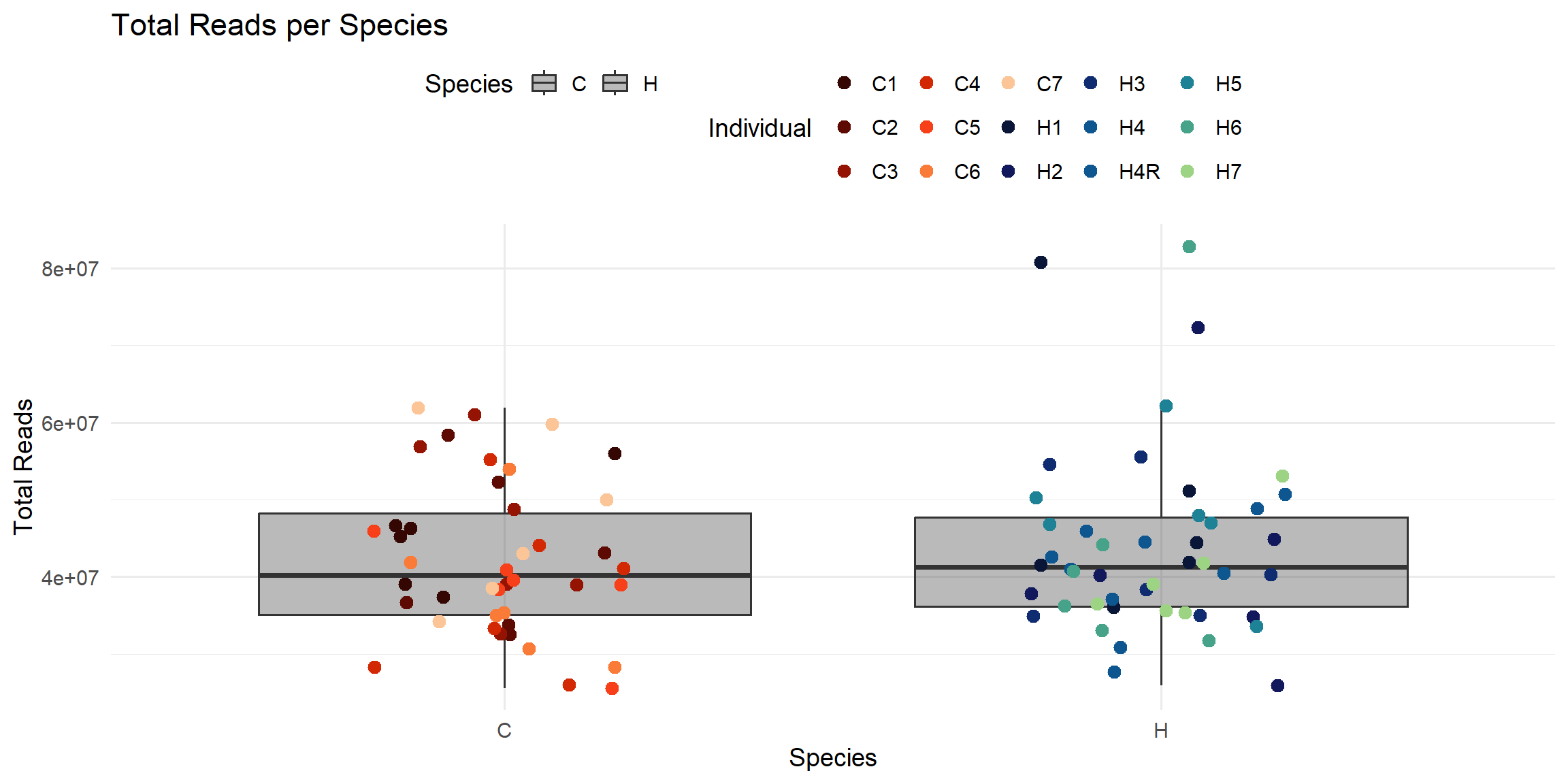
ggplot(total_reads_df, aes(x = Species, y = Total_Reads.x)) +
  
  # Boxplot for each species
  geom_boxplot(aes(fill = Species), alpha = 0.3, outlier.shape = NA) + 
  
  # Overlay individual points colored by individual
  geom_jitter(aes(color = Individual), width = 0.2, size = 3) +

  # Use individual colors
  scale_color_manual(values = ann_colors$individual_cor) +

  # Optional: species fill colors (light grey / black)
  scale_fill_manual(values = c("H" = "#17171717", "C" = "#17171717")) +

  theme_minimal(base_size = 14) +
  theme(
    legend.position = "top"
  ) +

  labs(
    title = "Total Reads per Species",
    x = "Species",
    y = "Total Reads",
    color = "Individual",
    fill = "Species"
  )

Past versions of RNASeq_TotalReads_graph-2.png

Version	Author	Date
0c9c163	John D. Hurley	2026-04-02

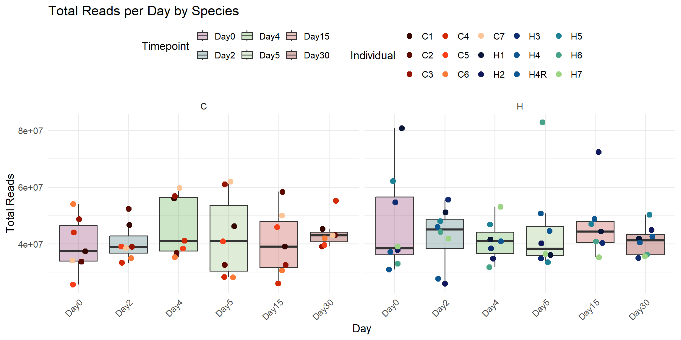
ggplot(total_reads_df, aes(x = Timepoint, y = Total_Reads.x)) +
  
  # Boxplot per day
  geom_boxplot(aes(fill = Timepoint), alpha = 0.3, outlier.shape = NA) +

  # Overlay individual points colored by individual
  geom_jitter(aes(color = Individual), width = 0.15, size = 3) +

  # Use individual colors
  scale_color_manual(values = ann_colors$individual_cor) +

  # Use timepoint colors for boxplots
  scale_fill_manual(values = ann_colors$timepoint_cor) +

  # Separate x-axis by species
  facet_wrap(~Species, scales = "free_x") +

  theme_minimal(base_size = 14) +
  theme(
    legend.position = "top",
    axis.text.x = element_text(angle = 45, hjust = 1)
  ) +

  labs(
    title = "Total Reads per Day by Species",
    x = "Day",
    y = "Total Reads",
    color = "Individual",
    fill = "Timepoint"
  )

Past versions of RNASeq_TotalReads_graph-3.png

Version	Author	Date
0c9c163	John D. Hurley	2026-04-02

# Plot
ggplot(total_reads_df, aes(x = Individual, y = Total_Reads.x)) +
  
  # Boxplots colored by individual
  geom_boxplot(aes(fill = Individual), alpha = 0.3, outlier.shape = NA) +

  # Overlay points colored by Timepoint
  geom_jitter(aes(color = Timepoint), width = 0.2, size = 3) +

  # Use manual colors
  scale_fill_manual(values = ann_colors$individual_cor) +
  scale_color_manual(values = ann_colors$timepoint_cor) +

  # Facet by species
  facet_wrap(~Species, scales = "free_x", nrow = 1) +

  # Theme
  theme_minimal(base_size = 14) +
  theme(
    legend.position = "top",
    axis.text.x = element_text(angle = 45, hjust = 1)
  ) +

  labs(
    title = "Total Reads per Individual by Species",
    x = "Individual",
    y = "Total Reads",
    fill = "Individual",
    color = "Timepoint"
  )

Past versions of RNASeq_TotalReads_graph-4.png

Version	Author	Date
0c9c163	John D. Hurley	2026-04-02

######Cor_HeatMap####
Cor_Filt_RMG0_RNA_log2cpm <- cor(Filt_RMG0_RNA_log2cpm, method = "spearman")
individual <- RNA_Metadata$Individual
species <- RNA_Metadata$Species
timepoint <- RNA_Metadata$Timepoint
timepoint <- factor(timepoint,levels = c("Day0","Day2","Day4","Day5","Day15","Day30"))
Cor_metadata <- data.frame(
  sample_cor = colnames(Filt_RMG0_RNA_log2cpm),
  species_cor = species,
  timepoint_cor = timepoint,
  individual_cor = individual
)


ann_colors <- list(
  timepoint_cor = c(
    "Day0" = "#883268",   # Purple
    "Day2" = "#3E7274",  # blue
    "Day4" = "#5AAA464D",  # light green
    "Day5" = "#94C47D",  # Green
    "Day15" = "#C03830",  # red
    "Day30" = "#830C05"  # dark red
  ),
  species_cor = c(
    "H" = "black",  # black
    "C" = "white"   # white
  ),
  individual_cor = c(
    H1 = "#091638", #Blue-Green Darkest
    H2 = "#11185B",
    H3 = "#0F2C71",
    H4 = "#0D568F",
    H4R = "#0D568F",
    H5 = "#1D8296",
    H6 = "#46A389",
    H7 = "#9DD484", #Blue-Green Lightest
    C1 = "#340702", #Brown-Orange darkest
    C2 = "#5D0B02",
    C3 = "#951302",
    C4 = "#D32804",
    C5 = "#F74019",
    C6 = "#FA7A38",
    C7 = "#FCC598"
    
  )
)
rownames(Cor_metadata) <- Cor_metadata$sample_cor

# saveRDS(Cor_Filt_RMG0_RNA_log2cpm, "data/QC/concat/Cor_Filt_RMG0_RNA_log2cpm.RDS")
# saveRDS(Cor_metadata, "data/QC/concat/Cor_RNA_metadata.RDS")
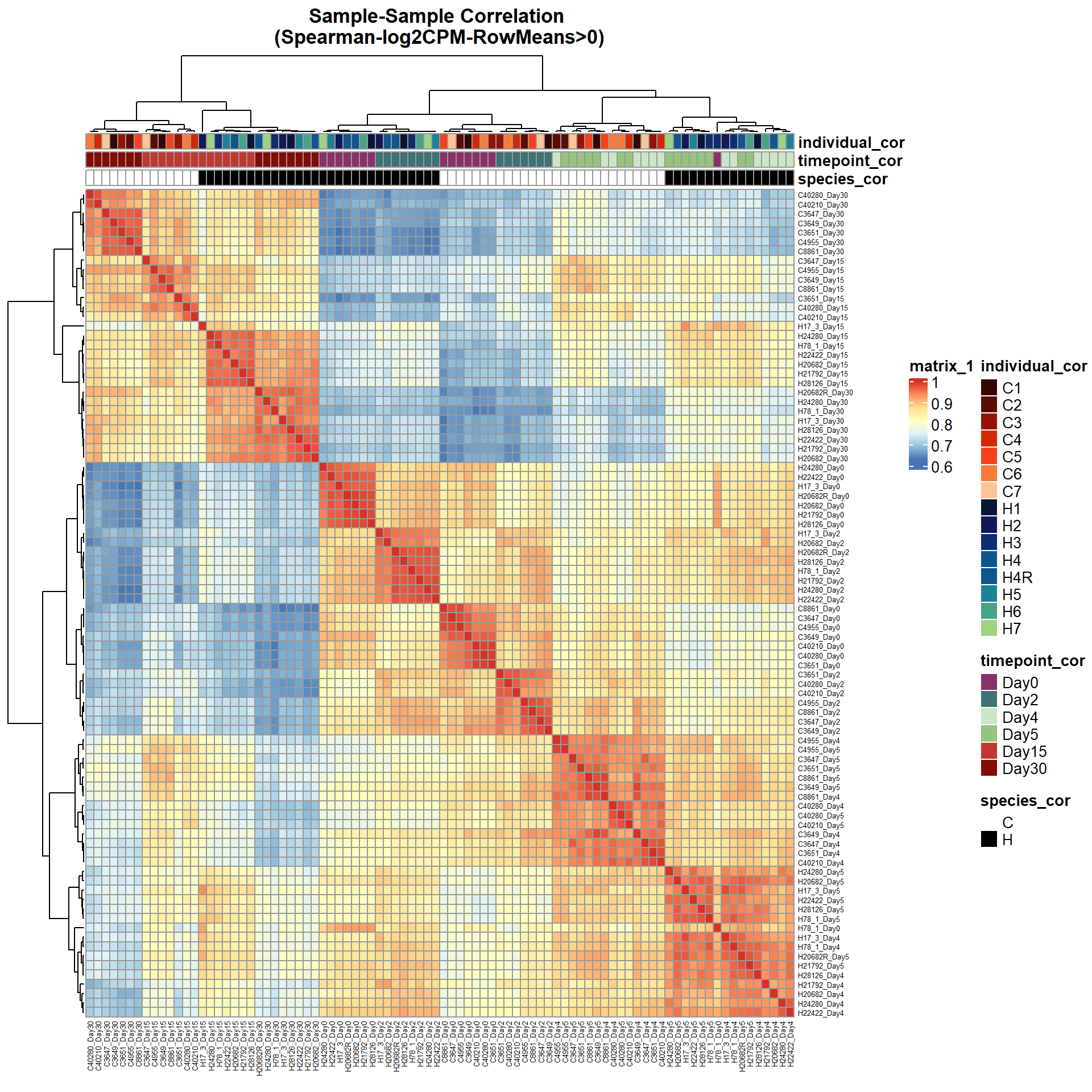
# saveRDS(ann_colors,"data/QC/concat/ann_colors.RDS")

print(
  pheatmap(Cor_Filt_RMG0_RNA_log2cpm,
         fontsize_row = 5,
         fontsize_col = 5,
         annotation_col = Cor_metadata[, c("species_cor", "timepoint_cor","individual_cor")],
         annotation_colors = ann_colors,
         clustering_distance_rows = "correlation",
         clustering_distance_cols = "correlation",
         main = "Sample-Sample Correlation \n(Spearman-log2CPM-RowMeans>0)")
)

Past versions of RNASeq_FeatureCounts_HeatMap_RMG0-1.png

Version	Author	Date
0c9c163	John D. Hurley	2026-04-02
0958201	John D. Hurley	2026-03-23
fcf8fc0	John D. Hurley	2026-02-18
7789dff	John D. Hurley	2026-01-28
d9f15a6	John D. Hurley	2026-01-28

####Subset####
RNA_Metadata_No4 <- RNA_Metadata %>% 
 filter(Timepoint != "Day4")

RNA_fc_NoD4 <- RNA_fc %>% 
  dplyr::select(-ends_with("_Day4"))

RNA_log2cpm_NoD4 <- cpm(RNA_fc_NoD4,log=TRUE)
dim(RNA_log2cpm_NoD4)

[1] 44125    74

dim(RNA_fc)

[1] 44125    88

row_means_NoD4 <- rowMeans(RNA_log2cpm_NoD4)
Filt_RMG0_RNA_fc_NoD4 <- RNA_fc_NoD4[row_means_NoD4 >0,]
dim(Filt_RMG0_RNA_fc_NoD4)

[1] 14084    74

Filt_RMG0_RNA_log2cpm_NoD4 <- cpm(Filt_RMG0_RNA_fc_NoD4,log=TRUE)

# saveRDS(RNA_Metadata_No4,"data/QC/concat/RNA_Metatdata_No4.RDS")
# saveRDS(Filt_RMG0_RNA_fc_NoD4,"data/QC/concat/Filt_RMG0_RNA_fc_NoD4.RDS")
# saveRDS(Filt_RMG0_RNA_log2cpm_NoD4, "data/QC/concat/Filt_RMG0_RNA_log2cpm_NoD4.RDS")

######Cor_HeatMap####
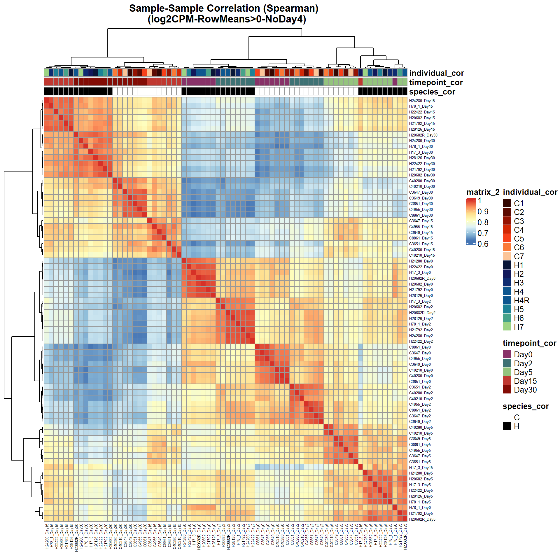
Cor_Filt_RMG0_RNA_log2cpm_NoD4 <- cor(Filt_RMG0_RNA_log2cpm_NoD4, method = "spearman")

Cor_metadata_No4 <- Cor_metadata %>% 
  dplyr::filter(timepoint_cor !="Day4")

ann_colors_No4 <- ann_colors
ann_colors_No4$timepoint_cor <- ann_colors$timepoint_cor[
  names(ann_colors$timepoint_cor) != "Day4"
]

# saveRDS(Cor_metadata_No4, "data/QC/concat/Cor_metadata_No4.RDS")
# saveRDS(Cor_Filt_RMG0_RNA_log2cpm_NoD4, "data/QC/concat/Cor_Filt_RMG0_RNA_log2cpm_NoD4.RDS")
# saveRDS(ann_colors_No4,"data/QC/concat/ann_colors_no4.RDS")

print(
  pheatmap(Cor_Filt_RMG0_RNA_log2cpm_NoD4,
         fontsize_row = 5,
         fontsize_col = 5,
         annotation_col = Cor_metadata_No4[, c("species_cor", "timepoint_cor","individual_cor")],
         annotation_colors = ann_colors_No4,
         clustering_distance_rows = "correlation",
         clustering_distance_cols = "correlation",
         main = "Sample-Sample Correlation (Spearman) \n (log2CPM-RowMeans>0-NoDay4)")
)

Past versions of rRNASeq_FeatureCounts_HeatMap_RMG0_No4-1.png

Version	Author	Date
0c9c163	John D. Hurley	2026-04-02
0958201	John D. Hurley	2026-03-23
fcf8fc0	John D. Hurley	2026-02-18
7789dff	John D. Hurley	2026-01-28
d9f15a6	John D. Hurley	2026-01-28

####Subset####
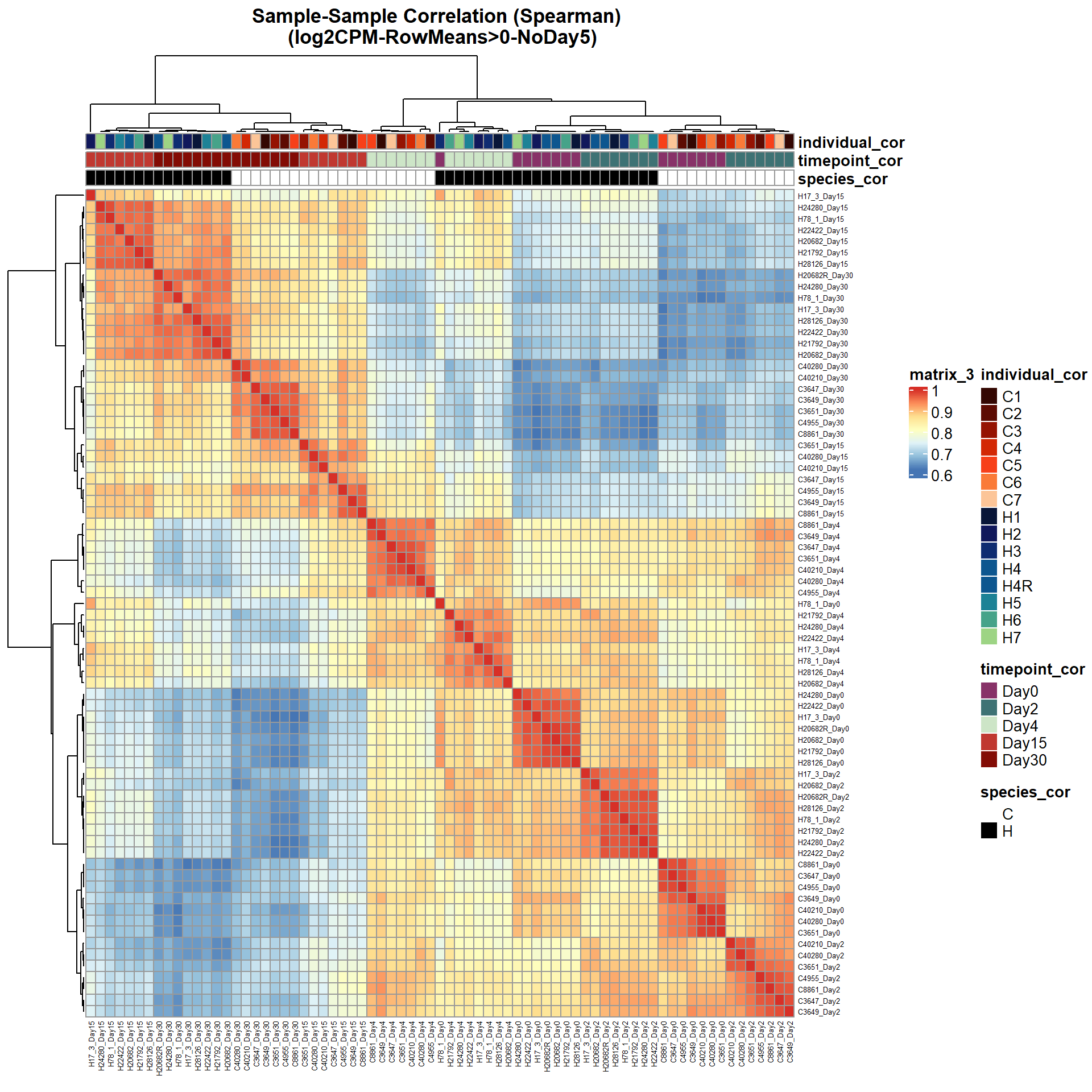
RNA_Metadata_No5 <- RNA_Metadata %>% 
 filter(Timepoint != "Day5")

RNA_fc_NoD5 <- RNA_fc %>% 
  dplyr::select(-ends_with("_Day5"))

RNA_log2cpm_NoD5 <- cpm(RNA_fc_NoD5,log=TRUE)
dim(RNA_log2cpm_NoD5)

[1] 44125    73

dim(RNA_fc)

[1] 44125    88

row_means_NoD5 <- rowMeans(RNA_log2cpm_NoD5)
Filt_RMG0_RNA_fc_NoD5 <- RNA_fc_NoD5[row_means_NoD5 >0,]
dim(Filt_RMG0_RNA_fc_NoD5)

[1] 14058    73

Filt_RMG0_RNA_log2cpm_NoD5 <- cpm(Filt_RMG0_RNA_fc_NoD5,log=TRUE)

# saveRDS(RNA_Metadata_No5,"data/QC/concat/RNA_Metatdata_No5.RDS")
# saveRDS(Filt_RMG0_RNA_fc_NoD5,"data/QC/concat/Filt_RMG0_RNA_fc_NoD5.RDS")
# saveRDS(Filt_RMG0_RNA_log2cpm_NoD5, "data/QC/concat/Filt_RMG0_RNA_log2cpm_NoD5.RDS")

######Cor_HeatMap####
Cor_Filt_RMG0_RNA_log2cpm_NoD5 <- cor(Filt_RMG0_RNA_log2cpm_NoD5, method = "spearman")

Cor_metadata_No5 <- Cor_metadata %>% 
  dplyr::filter(timepoint_cor !="Day5")

ann_colors_No5 <- ann_colors
ann_colors_No5$timepoint_cor <- ann_colors$timepoint_cor[
  names(ann_colors$timepoint_cor) != "Day5"
]

# saveRDS(Cor_metadata_No5, "data/QC/concat/Cor_metadata_No5.RDS")
# saveRDS(Cor_Filt_RMG0_RNA_log2cpm_NoD5, "data/QC/concat/Cor_Filt_RMG0_RNA_log2cpm_NoD5.RDS")
# saveRDS(ann_colors_No5,"data/QC/concat/ann_colors_no5.RDS")

print(
  pheatmap(Cor_Filt_RMG0_RNA_log2cpm_NoD5,
         fontsize_row = 5,
         fontsize_col = 5,
         annotation_col = Cor_metadata_No5[, c("species_cor", "timepoint_cor","individual_cor")],
         annotation_colors = ann_colors_No5,
         clustering_distance_rows = "correlation",
         clustering_distance_cols = "correlation",
         main = "Sample-Sample Correlation (Spearman) \n (log2CPM-RowMeans>0-NoDay5)")
)

Past versions of rRNASeq_FeatureCounts_HeatMap_RMG0_No5-1.png

Version	Author	Date
0c9c163	John D. Hurley	2026-04-02

markers <- marker_genes$Ensembl.ID

log2cpm_long <- RNA_log2cpm %>%
  as.data.frame() %>%
  rownames_to_column("Ensembl.ID") %>%
  filter(Ensembl.ID %in% markers) %>% 
  pivot_longer(
    cols = -Ensembl.ID,
    names_to = "Sample",
    values_to = "log2CPM"
  )

log2cpm_long <- log2cpm_long %>%
  left_join(RNA_Metadata, by = c("Sample" = "SampleName"))

log2cpm_long <- log2cpm_long %>%
  left_join(marker_genes, by = "Ensembl.ID")

log2cpm_long$Timepoint <- factor(
  log2cpm_long$Timepoint,
  levels = c("Day0", "Day2", "Day4", "Day5", "Day15", "Day30")
)

log2cpm_long_NoR <- log2cpm_long %>% 
  filter(Individual != "H4R")

library(dplyr)

mean_df <- log2cpm_long_NoR %>%
  group_by(Stage, Timepoint, Species) %>%
  summarise(
    mean_log2CPM = mean(log2CPM),
    .groups = "drop"
  )

log2cpm_long_NoR$Stage <- factor(
  log2cpm_long_NoR$Stage,
  levels = c(
    "Pluripotency",
    "Mesoderm",
    "CardiacMesoderm",
    "CardiacProgenitors",
    "EarlyCardiomyocytes",
    "MatureCardiomyocytes"
  )
)

library(ggplot2)

ggplot(log2cpm_long_NoR, aes(
  x = Timepoint,
  y = log2CPM
)) +

  geom_boxplot(
    aes(fill = Stage),
    alpha = 0.3,
    outlier.shape = NA
  ) +

  geom_line(
    data = mean_df,
    aes(
      x = Timepoint,
      y = mean_log2CPM,
      group = interaction(Stage, Species),
      linetype = Species
    ),
    color = "black",
    linewidth = 1.2
  ) +

  geom_point(
    data = mean_df,
    aes(
      x = Timepoint,
      y = mean_log2CPM,
      shape = Species
    ),
    color = "black",
    size = 2
  ) +

  scale_linetype_manual(values = c(
    C = "dotted",
    H = "solid"
  )) +

  scale_shape_manual(values = c(
    C = 16,
    H = 17
  )) +

  facet_wrap(~ factor(Stage, levels = levels(log2cpm_long_NoR$Stage))) +
  theme_classic() +
  theme(axis.text.x = element_text(angle = 45, hjust = 1))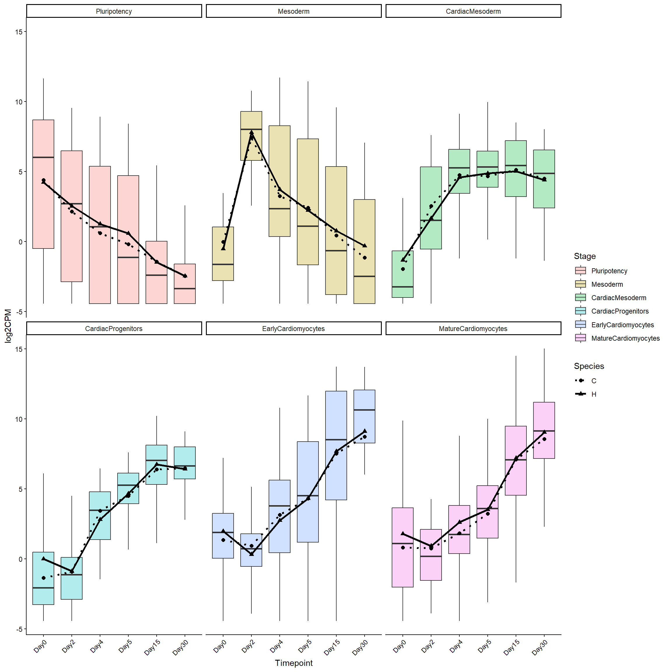

Past versions of RNASeq_MarkerGenes_graph-1.png

Version	Author	Date
0c9c163	John D. Hurley	2026-04-02
9d3ae04	John D. Hurley	2026-03-30

library(ggplot2)

ggplot(log2cpm_long_NoR, aes(
  x = Timepoint,
  y = log2CPM
)) +

  geom_boxplot(
  aes(fill = Species, group = interaction(Timepoint, Species)),
  alpha = 0.3,
  outlier.shape = NA,
  position = position_dodge(width = 0.8)
  ) +
  
    scale_fill_manual(values = ann_colors$species_cor) +
  
    geom_jitter(
  aes(color = Individual),
  position = position_jitterdodge(
    jitter.width = 0.15,
    dodge.width = 0.8
  ),
  size = 1,
  alpha = 0.6
) +
  
  scale_color_manual(values = ann_colors$individual_cor)+

  geom_line(
    data = mean_df,
    aes(
      x = Timepoint,
      y = mean_log2CPM,
      group = interaction(Stage, Species),
      linetype = Species
    ),
    color = "black",
    linewidth = 1.2
  ) +

  geom_point(
    data = mean_df,
    aes(
      x = Timepoint,
      y = mean_log2CPM,
      shape = Species
    ),
    color = "black",
    size = 2
  ) +

  scale_linetype_manual(values = c(
    C = "dotted",
    H = "solid"
  )) +

  scale_shape_manual(values = c(
    C = 16,
    H = 17
  )) +

  facet_wrap(~ factor(Stage, levels = levels(log2cpm_long_NoR$Stage))) +
  theme_classic() +
  theme(axis.text.x = element_text(angle = 45, hjust = 1))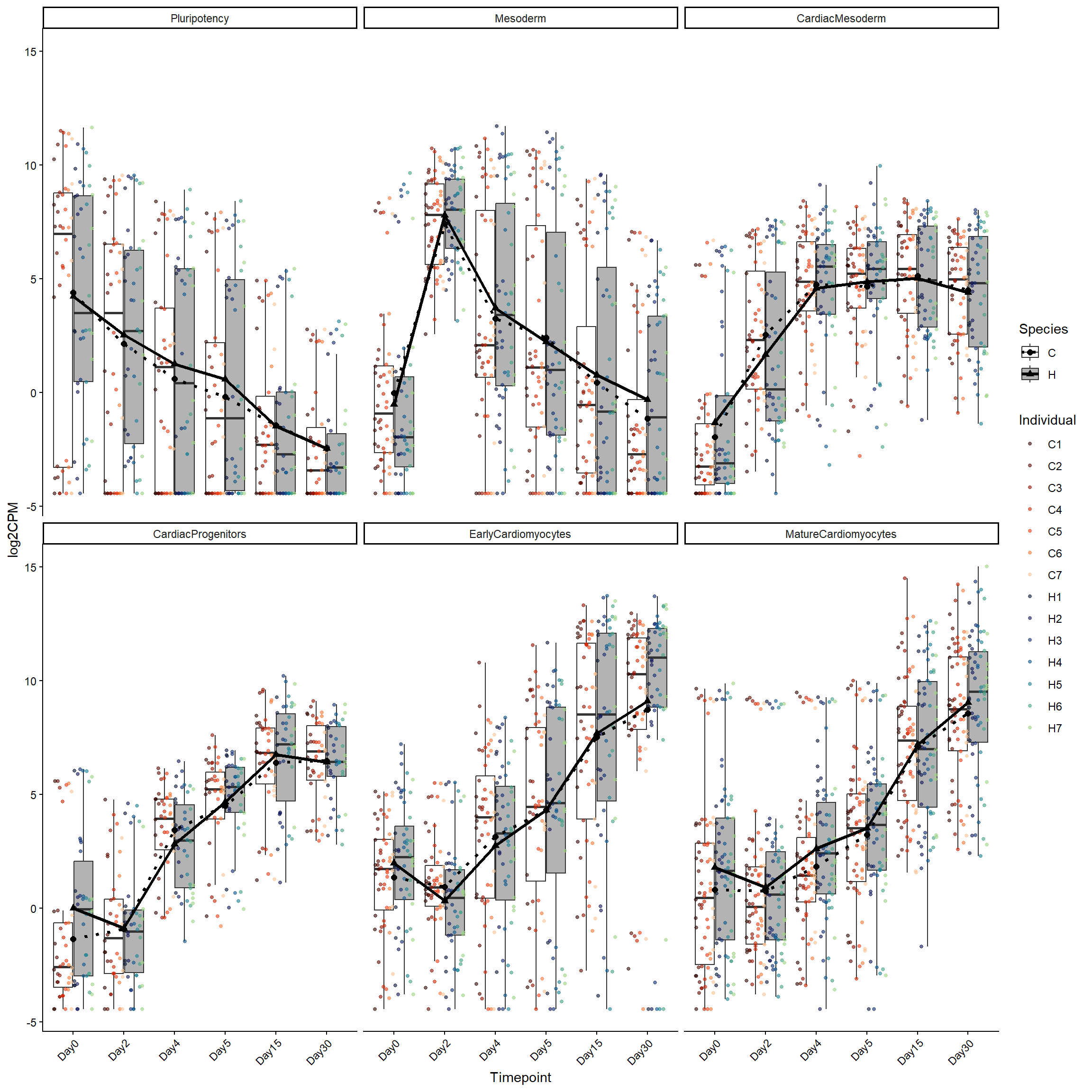

Past versions of RNASeq_MarkerGenes_graph_species_separated-1.png

Version	Author	Date
0c9c163	John D. Hurley	2026-04-02

pluri_genes <- log2cpm_long_NoR %>%
  filter(Stage == "Pluripotency")

ggplot(pluri_genes, aes(x = Timepoint, y = log2CPM)) +

  geom_boxplot(
    aes(fill = Species, group = interaction(Timepoint, Species)),
    position = position_dodge(width = 0.8),
    alpha = 0.3,
    outlier.shape = NA
  ) +
  
      scale_fill_manual(values = ann_colors$species_cor) +
  
     geom_jitter(
  aes(color = Individual),
  position = position_jitterdodge(
    jitter.width = 0.15,
    dodge.width = 0.8
  ),
  size = 3,
  alpha = 0.6
) +
  
  scale_color_manual(values = ann_colors$individual_cor)+

  geom_line(
    stat = "summary",
    fun = mean,
    aes(group = Species, linetype = Species),
    position = position_dodge(width = 0.8),
    linewidth = 1
  ) +
  
    scale_linetype_manual(values = c(
    C = "dotted",
    H = "solid"
  )) +

  geom_point(
    stat = "summary",
    fun = mean,
    aes(shape = Species),
    position = position_dodge(width = 0.8),
    size = 2
  ) +

  facet_wrap(~ Gene, scales = "free_y") +

  theme_classic() +
  theme(axis.text.x = element_text(angle = 45, hjust = 1))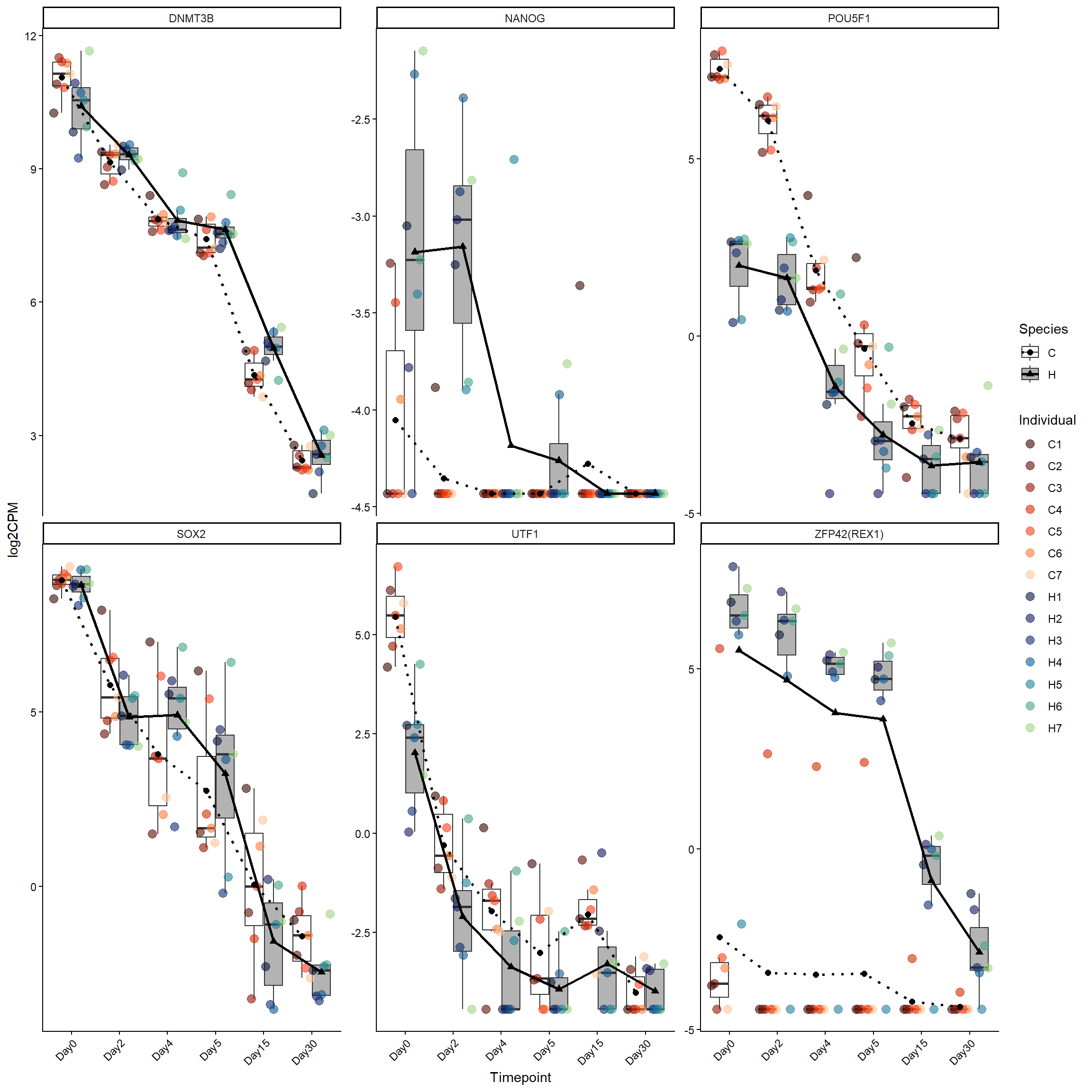

Past versions of RNASeq_MarkerGenes_graph_species_separated_pluri-1.png

Version	Author	Date
0c9c163	John D. Hurley	2026-04-02

meso_genes <- log2cpm_long_NoR %>%
  filter(Stage == "Mesoderm")

ggplot(meso_genes, aes(x = Timepoint, y = log2CPM)) +

  geom_boxplot(
    aes(fill = Species, group = interaction(Timepoint, Species)),
    position = position_dodge(width = 0.8),
    alpha = 0.3,
    outlier.shape = NA
  ) +
  
      scale_fill_manual(values = ann_colors$species_cor) +

    geom_jitter(
  aes(color = Individual),
  position = position_jitterdodge(
    jitter.width = 0.15,
    dodge.width = 0.8
  ),
  size = 1,
  alpha = 0.6
) +
  
  scale_color_manual(values = ann_colors$individual_cor)+
  
  geom_line(
    stat = "summary",
    fun = mean,
    aes(group = Species, linetype = Species),
    position = position_dodge(width = 0.8),
    linewidth = 1
  ) +
  
    scale_linetype_manual(values = c(
    C = "dotted",
    H = "solid"
  )) +

  geom_point(
    stat = "summary",
    fun = mean,
    aes(shape = Species),
    position = position_dodge(width = 0.8),
    size = 2
  ) +

  facet_wrap(~ Gene, scales = "free_y") +

  theme_classic() +
  theme(axis.text.x = element_text(angle = 45, hjust = 1))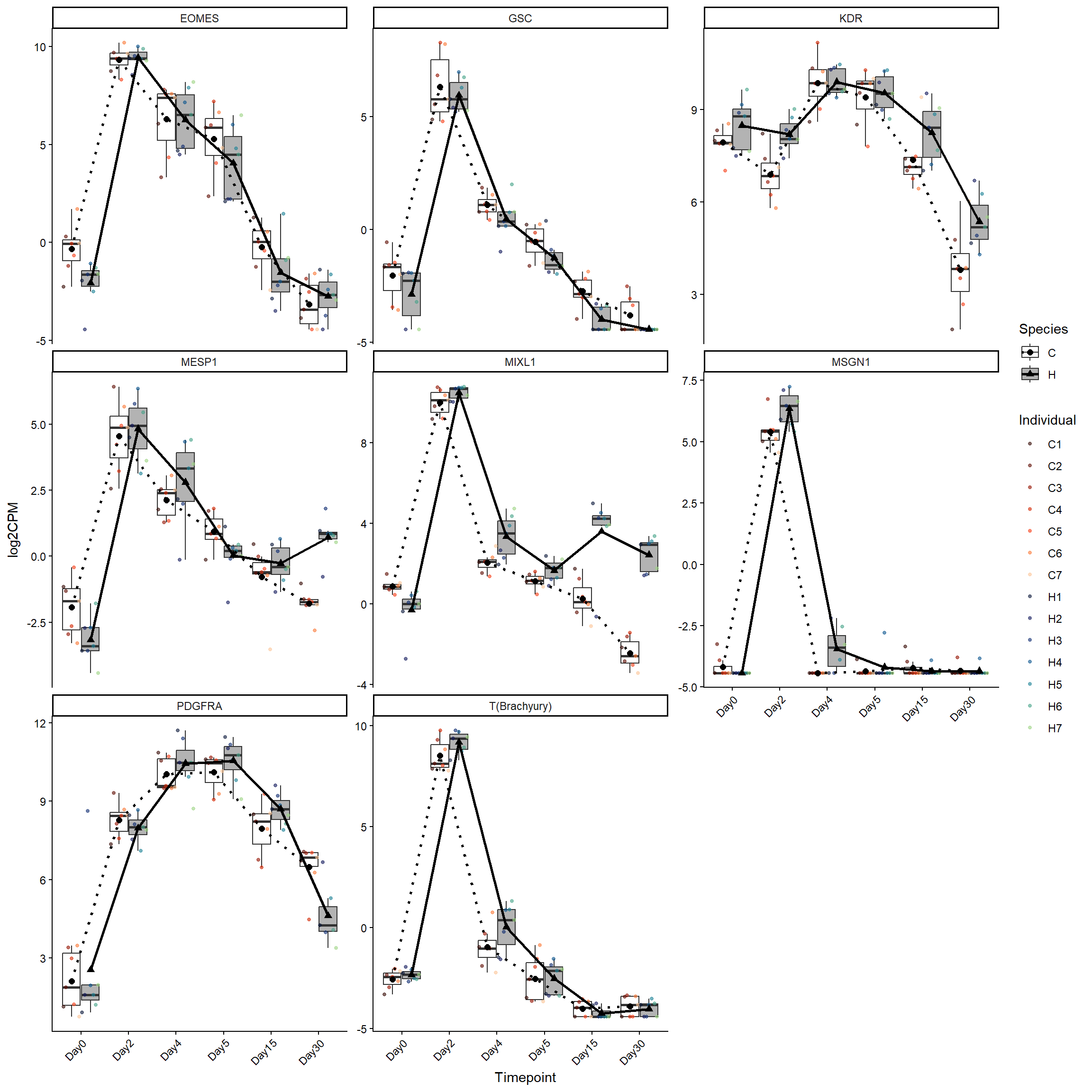

Past versions of RNASeq_MarkerGenes_graph_species_separated_meso-1.png

Version	Author	Date
0c9c163	John D. Hurley	2026-04-02

cardmeso_genes <- log2cpm_long_NoR %>%
  filter(Stage == "CardiacMesoderm")

ggplot(cardmeso_genes, aes(x = Timepoint, y = log2CPM)) +

  geom_boxplot(
    aes(fill = Species, group = interaction(Timepoint, Species)),
    position = position_dodge(width = 0.8),
    alpha = 0.3,
    outlier.shape = NA
  ) +
  
      scale_fill_manual(values = ann_colors$species_cor) +
  
  
    geom_jitter(
  aes(color = Individual),
  position = position_jitterdodge(
    jitter.width = 0.15,
    dodge.width = 0.8
  ),
  size = 1,
  alpha = 0.6
) +
  
  scale_color_manual(values = ann_colors$individual_cor)+
  geom_line(
    stat = "summary",
    fun = mean,
    aes(group = Species, linetype = Species),
    position = position_dodge(width = 0.8),
    linewidth = 1
  ) +
  
    scale_linetype_manual(values = c(
    C = "dotted",
    H = "solid"
  )) +

  geom_point(
    stat = "summary",
    fun = mean,
    aes(shape = Species),
    position = position_dodge(width = 0.8),
    size = 2
  ) +

  facet_wrap(~ Gene, scales = "free_y") +

  theme_classic() +
  theme(axis.text.x = element_text(angle = 45, hjust = 1))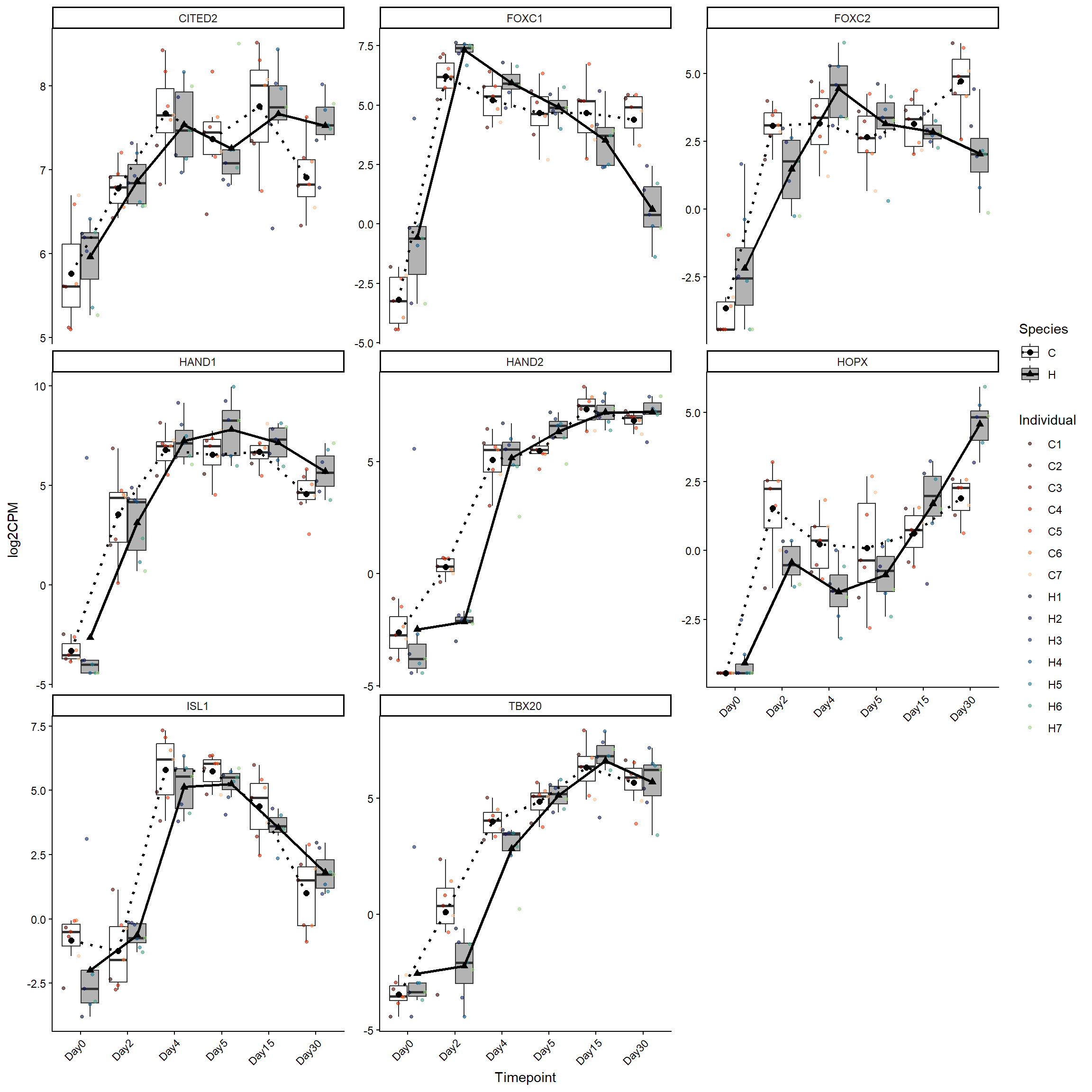

Past versions of RNASeq_MarkerGenes_graph_species_separated_cardmeso-1.png

Version	Author	Date
0c9c163	John D. Hurley	2026-04-02

cardprog_genes <- log2cpm_long_NoR %>%
  filter(Stage == "CardiacProgenitors")

ggplot(cardprog_genes, aes(x = Timepoint, y = log2CPM)) +

  geom_boxplot(
    aes(fill = Species, group = interaction(Timepoint, Species)),
    position = position_dodge(width = 0.8),
    alpha = 0.3,
    outlier.shape = NA
  ) +
  
      scale_fill_manual(values = ann_colors$species_cor) +
  
    geom_jitter(
  aes(color = Individual),
  position = position_jitterdodge(
    jitter.width = 0.15,
    dodge.width = 0.8
  ),
  size = 1,
  alpha = 0.6
) +
  
  scale_color_manual(values = ann_colors$individual_cor)+

  geom_line(
    stat = "summary",
    fun = mean,
    aes(group = Species, linetype = Species),
    position = position_dodge(width = 0.8),
    linewidth = 1
  ) +
  
    scale_linetype_manual(values = c(
    C = "dotted",
    H = "solid"
  )) +

  geom_point(
    stat = "summary",
    fun = mean,
    aes(shape = Species),
    position = position_dodge(width = 0.8),
    size = 2
  ) +

  facet_wrap(~ Gene, scales = "free_y") +

  theme_classic() +
  theme(axis.text.x = element_text(angle = 45, hjust = 1))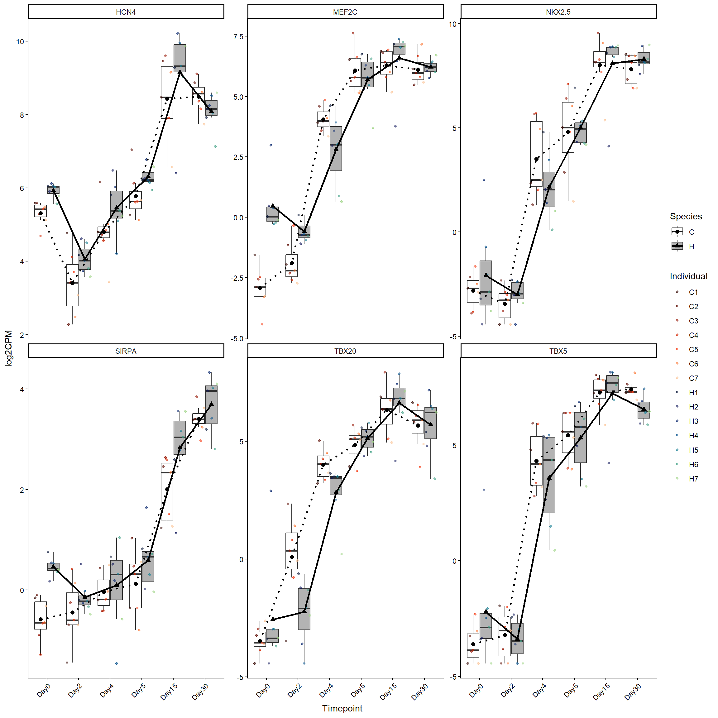

Past versions of RNASeq_MarkerGenes_graph_species_separated_cardprog-1.png

Version	Author	Date
0c9c163	John D. Hurley	2026-04-02

cardearly_genes <- log2cpm_long_NoR %>%
  filter(Stage == "EarlyCardiomyocytes")

ggplot(cardearly_genes, aes(x = Timepoint, y = log2CPM)) +

  geom_boxplot(
    aes(fill = Species, group = interaction(Timepoint, Species)),
    position = position_dodge(width = 0.8),
    alpha = 0.3,
    outlier.shape = NA
  ) +
  
      scale_fill_manual(values = ann_colors$species_cor) +
  
  
    geom_jitter(
  aes(color = Individual),
  position = position_jitterdodge(
    jitter.width = 0.15,
    dodge.width = 0.8
  ),
  size = 1,
  alpha = 0.6
) +
  
  scale_color_manual(values = ann_colors$individual_cor)+

  geom_line(
    stat = "summary",
    fun = mean,
    aes(group = Species, linetype = Species),
    position = position_dodge(width = 0.8),
    linewidth = 1
  ) +
  
    scale_linetype_manual(values = c(
    C = "dotted",
    H = "solid"
  )) +

  geom_point(
    stat = "summary",
    fun = mean,
    aes(shape = Species),
    position = position_dodge(width = 0.8),
    size = 2
  ) +

  facet_wrap(~ Gene, scales = "free_y") +

  theme_classic() +
  theme(axis.text.x = element_text(angle = 45, hjust = 1))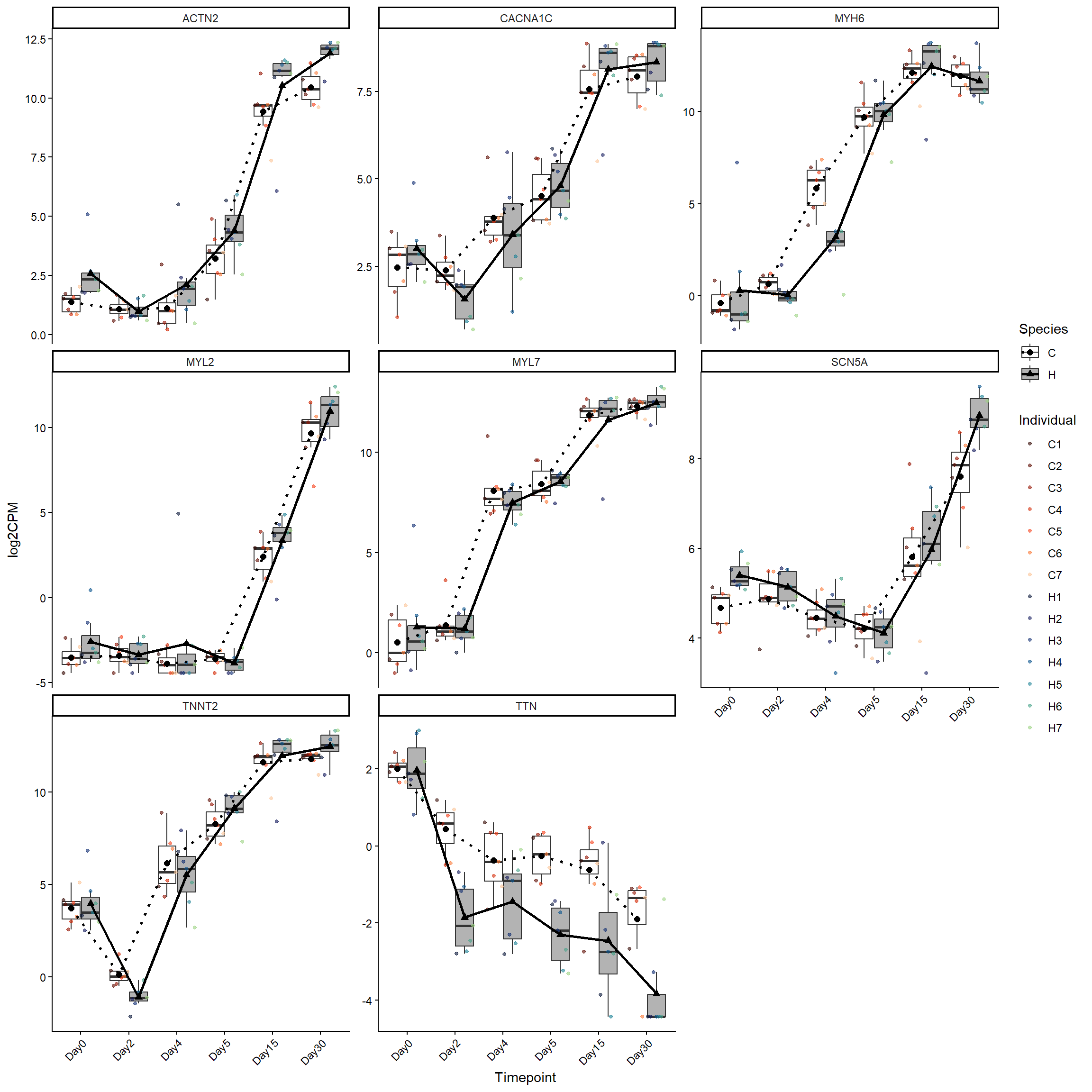

Past versions of RNASeq_MarkerGenes_graph_species_separated_cardearly-1.png

Version	Author	Date
0c9c163	John D. Hurley	2026-04-02

cardlate_genes <- log2cpm_long_NoR %>%
  filter(Stage == "MatureCardiomyocytes")

ggplot(cardlate_genes, aes(x = Timepoint, y = log2CPM)) +

  geom_boxplot(
    aes(fill = Species, group = interaction(Timepoint, Species)),
    position = position_dodge(width = 0.8),
    alpha = 0.3,
    outlier.shape = NA
  ) +

  scale_fill_manual(values = ann_colors$species_cor) +
  
    geom_jitter(
  aes(color = Individual),
  position = position_jitterdodge(
    jitter.width = 0.15,
    dodge.width = 0.8
  ),
  size = 1,
  alpha = 0.6
) +
  
  scale_color_manual(values = ann_colors$individual_cor)+
  
  geom_line(
    stat = "summary",
    fun = mean,
    aes(group = Species, linetype = Species),
    position = position_dodge(width = 0.8),
    linewidth = 1
  ) +
  
    scale_linetype_manual(values = c(
    C = "dotted",
    H = "solid"
  )) +

  geom_point(
    stat = "summary",
    fun = mean,
    aes(shape = Species),
    position = position_dodge(width = 0.8),
    size = 2
  ) +

  facet_wrap(~ Gene, scales = "free_y") +

  theme_classic() +
  theme(axis.text.x = element_text(angle = 45, hjust = 1))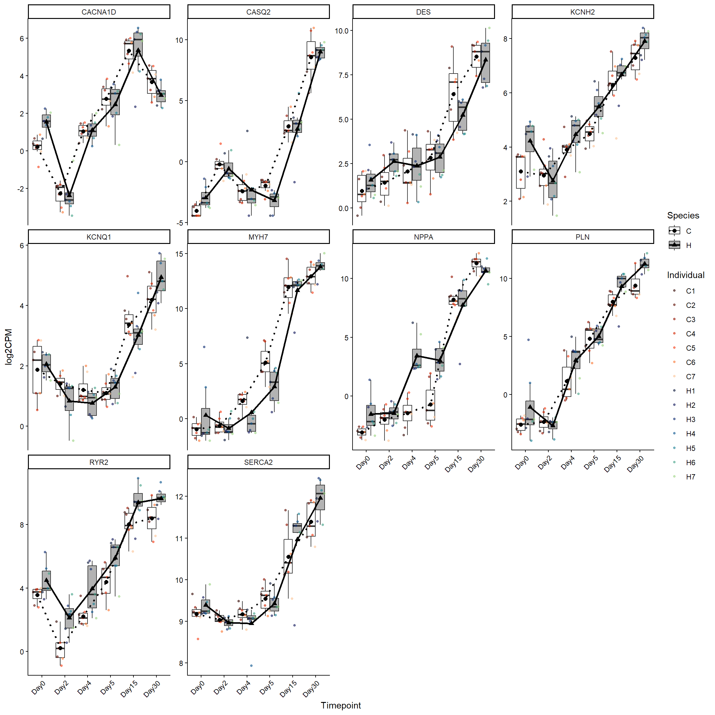

Past versions of RNASeq_MarkerGenes_graph_species_separated_cardlate-1.png

Version	Author	Date
0c9c163	John D. Hurley	2026-04-02

counts_table_genes <- unique(counts_table$Geneid)
Expressed_Genes <- unique(TopTable_RNA_All$Gene)
marker_genes_ortho <- marker_genes %>% 
  filter(Ensembl.ID %in% counts_table_genes)
marker_genes_ortho_expressed <- marker_genes_ortho %>% 
  filter(Ensembl.ID %in% Expressed_Genes)

# git -> commit all changes
# git -> push
wflow_publish("analysis/RNA_CorrelationHeatMap_Ensemble.Rmd")

Session information

sessionInfo()

R version 4.5.1 (2025-06-13 ucrt)
Platform: x86_64-w64-mingw32/x64
Running under: Windows 11 x64 (build 26100)

Matrix products: default
  LAPACK version 3.12.1

locale:
[1] LC_COLLATE=English_United States.utf8 
[2] LC_CTYPE=English_United States.utf8   
[3] LC_MONETARY=English_United States.utf8
[4] LC_NUMERIC=C                          
[5] LC_TIME=English_United States.utf8    

time zone: America/Chicago
tzcode source: internal

attached base packages:
[1] grid      stats4    stats     graphics  grDevices utils     datasets 
[8] methods   base     

other attached packages:
 [1] scales_1.4.0                ComplexHeatmap_2.24.1      
 [3] ggfortify_0.4.19            readxl_1.4.5               
 [5] RUVSeq_1.42.0               EDASeq_2.42.0              
 [7] ShortRead_1.66.0            GenomicAlignments_1.44.0   
 [9] SummarizedExperiment_1.38.1 MatrixGenerics_1.20.0      
[11] matrixStats_1.5.0           Rsamtools_2.24.0           
[13] GenomicRanges_1.60.0        Biostrings_2.76.0          
[15] GenomeInfoDb_1.44.3         XVector_0.48.0             
[17] BiocParallel_1.42.1         lubridate_1.9.5            
[19] forcats_1.0.1               stringr_1.6.0              
[21] purrr_1.2.1                 tidyr_1.3.2                
[23] tidyverse_2.0.0             Cormotif_1.54.0            
[25] affy_1.86.0                 pheatmap_1.0.13            
[27] org.Hs.eg.db_3.21.0         AnnotationDbi_1.70.0       
[29] IRanges_2.42.0              S4Vectors_0.46.0           
[31] Biobase_2.68.0              BiocGenerics_0.54.1        
[33] generics_0.1.4              readr_2.1.6                
[35] ggrepel_0.9.6               dplyr_1.1.4                
[37] tibble_3.3.1                ggplot2_4.0.2              
[39] edgeR_4.6.3                 limma_3.64.3               
[41] workflowr_1.7.2            

loaded via a namespace (and not attached):
  [1] later_1.4.5             BiocIO_1.18.0           bitops_1.0-9           
  [4] filelock_1.0.3          R.oo_1.27.1             cellranger_1.1.0       
  [7] preprocessCore_1.70.0   XML_3.99-0.20           lifecycle_1.0.5        
 [10] httr2_1.2.2             pwalign_1.4.0           doParallel_1.0.17      
 [13] rprojroot_2.1.1         processx_3.8.6          lattice_0.22-7         
 [16] MASS_7.3-65             magrittr_2.0.4          sass_0.4.10            
 [19] rmarkdown_2.31          jquerylib_0.1.4         yaml_2.3.12            
 [22] httpuv_1.6.16           otel_0.2.0              DBI_1.3.0              
 [25] RColorBrewer_1.1-3      abind_1.4-8             R.utils_2.13.0         
 [28] RCurl_1.98-1.18         rappdirs_0.3.4          git2r_0.36.2           
 [31] circlize_0.4.17         GenomeInfoDbData_1.2.14 codetools_0.2-20       
 [34] DelayedArray_0.34.1     xml2_1.5.2              tidyselect_1.2.1       
 [37] shape_1.4.6.1           UCSC.utils_1.4.0        farver_2.1.2           
 [40] BiocFileCache_2.16.2    jsonlite_2.0.0          GetoptLong_1.1.0       
 [43] iterators_1.0.14        foreach_1.5.2           tools_4.5.1            
 [46] progress_1.2.3          Rcpp_1.1.1              glue_1.8.0             
 [49] gridExtra_2.3           SparseArray_1.8.1       xfun_0.56              
 [52] withr_3.0.2             BiocManager_1.30.27     fastmap_1.2.0          
 [55] latticeExtra_0.6-31     callr_3.7.6             digest_0.6.39          
 [58] timechange_0.4.0        R6_2.6.1                colorspace_2.1-2       
 [61] Cairo_1.7-0             jpeg_0.1-11             biomaRt_2.64.0         
 [64] RSQLite_2.4.5           R.methodsS3_1.8.2       rtracklayer_1.68.0     
 [67] prettyunits_1.2.0       httr_1.4.8              S4Arrays_1.8.1         
 [70] whisker_0.4.1           pkgconfig_2.0.3         gtable_0.3.6           
 [73] blob_1.3.0              S7_0.2.1                hwriter_1.3.2.1        
 [76] htmltools_0.5.9         clue_0.3-68             png_0.1-8              
 [79] knitr_1.51              rstudioapi_0.18.0       tzdb_0.5.0             
 [82] rjson_0.2.23            curl_7.0.0              cachem_1.1.0           
 [85] GlobalOptions_0.1.3     parallel_4.5.1          restfulr_0.0.16        
 [88] pillar_1.11.1           vctrs_0.7.1             promises_1.5.0         
 [91] dbplyr_2.5.2            cluster_2.1.8.1         evaluate_1.0.5         
 [94] GenomicFeatures_1.60.0  cli_3.6.5               locfit_1.5-9.12        
 [97] compiler_4.5.1          rlang_1.1.7             crayon_1.5.3           
[100] labeling_0.4.3          interp_1.1-6            aroma.light_3.38.0     
[103] ps_1.9.1                getPass_0.2-4           fs_1.6.6               
[106] stringi_1.8.7           deldir_2.0-4            Matrix_1.7-4           
[109] hms_1.1.4               bit64_4.6.0-1           KEGGREST_1.48.1        
[112] statmod_1.5.1           memoise_2.0.1           affyio_1.78.0          
[115] bslib_0.10.0            bit_4.6.0